Practice Practice Page 170 6 10 How strong

Practice • Practice – Page 170 #6. 10 – How strong is the relationship?

Results X 2 = 5. 38 X 2 crit = 3. 83 ADD English

Phi • Use with 2 x 2 tables

2 as a test for goodness of fit • But what if: • You have a theory or hypothesis that the frequencies should occur in a particular manner?

Example • • M&Ms claim that of their candies: 30% are brown 20% are red 20% are yellow 10% are blue 10% are orange 10% are green

Example • Based on genetic theory you hypothesize that in the population: • 45% have brown eyes • 35% have blue eyes • 20% have another eye color

To solve you use the same basic steps as before (slightly • • different order) 1) State the hypothesis 2) Find 2 critical 3) Create data table 4) Calculate the expected frequencies 5) Calculate 2 6) Decision 7) Put answer into words

Example • M&Ms claim that of their candies: • • • 30% are brown 20% are red 20% are yellow 10% are blue 10% are orange 10% are green

Example • Four 1 -pound bags of plain M&Ms are purchased • Each M&Ms is counted and categorized according to its color • Question: Is M&Ms “theory” about the colors of M&Ms correct?

Step 1: State the Hypothesis • H 0: The data do fit the model – i. e. , the observed data does agree with M&M’s theory • H 1: The data do not fit the model – i. e. , the observed data does not agree with M&M’s theory – NOTE: These are backwards from what you have done before

Step 2: Find 2 critical • df = number of categories - 1

Step 2: Find 2 critical • df = number of categories - 1 • df = 6 - 1 = 5 • =. 05 • 2 critical = 11. 07

Step 3: Create the data table

Step 3: Create the data table Add the expected proportion of each category

Step 4: Calculate the Expected Frequencies

Step 4: Calculate the Expected Frequencies Expected Frequency = (proportion)(N)

Step 4: Calculate the Expected Frequencies Expected Frequency = (. 30)(2081) = 624. 30

Step 4: Calculate the Expected Frequencies Expected Frequency = (. 20)(2081) = 416. 20

Step 4: Calculate the Expected Frequencies Expected Frequency = (. 20)(2081) = 416. 20

Step 4: Calculate the Expected Frequencies Expected Frequency = (. 10)(2081) = 208. 10

Step 5: Calculate 2 O = observed frequency E = expected frequency

2

2

2

2

2

2 15. 52

Step 6: Decision • Thus, if 2 > than 2 critical – Reject H 0, and accept H 1 • If 2 < or = to 2 critical – Fail to reject H 0

Step 6: Decision • Thus, if 2 > than 2 critical – Reject H 0, and accept H 1 • If 2 < or = to 2 critical – Fail to reject H 0 2 = 15. 52 2 crit = 11. 07

Step 7: Put it answer into words • H 1: The data do not fit the model • M&M’s color “theory” did not significantly (. 05) fit the data

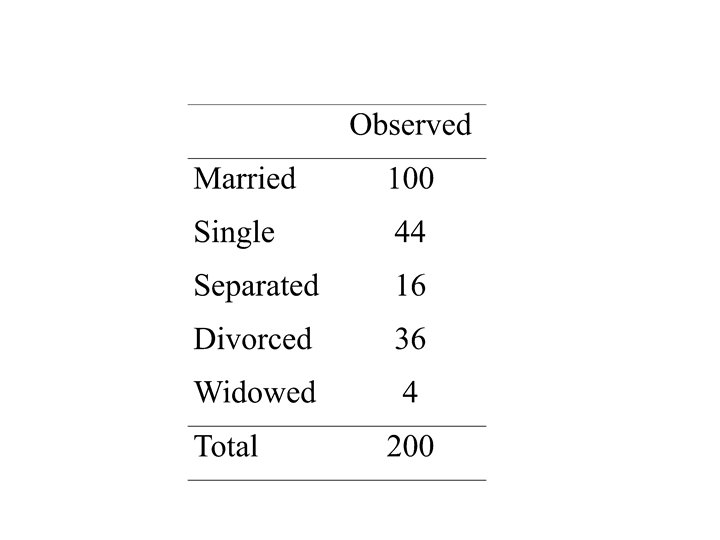
Practice • Among women in the general population under the age of 40: • • • 60% are married 23% are single 4% are separated 12% are divorced 1% are widowed

Practice • You sample 200 female executives under the age of 40 • Question: Is marital status distributed the same way in the population of female executives as in the general population ( =. 05)?

Step 1: State the Hypothesis • H 0: The data do fit the model – i. e. , marital status is distributed the same way in the population of female executives as in the general population • H 1: The data do not fit the model – i. e. , marital status is not distributed the same way in the population of female executives as in the general population

Step 2: Find 2 critical • df = number of categories - 1

Step 2: Find 2 critical • df = number of categories - 1 • df = 5 - 1 = 4 • =. 05 • 2 critical = 9. 49

Step 3: Create the data table

Step 4: Calculate the Expected Frequencies

Step 5: Calculate 2 O = observed frequency E = expected frequency

2 19. 42

Step 6: Decision • Thus, if 2 > than 2 critical – Reject H 0, and accept H 1 • If 2 < or = to 2 critical – Fail to reject H 0

Step 6: Decision • Thus, if 2 > than 2 critical – Reject H 0, and accept H 1 • If 2 < or = to 2 critical – Fail to reject H 0 2 = 19. 42 2 crit = 9. 49

Step 7: Put it answer into words • H 1: The data do not fit the model • Marital status is not distributed the same way in the population of female executives as in the general population ( =. 05)

Practice • In the past you have had a 20% success rate at getting someone to accept a date from you. • What is the probability that at least 2 of the next 10 people you ask out will accept?

Practice • p zero will accept =. 11 • p one will accept =. 27 • p zero OR one will accept =. 38 • p two or more will accept = 1 -. 38 =. 62

Practice • IQ – Mean = 100 – SD = 15 • What is the probability that the stranger you just bumped into on the street has an IQ between 95 and 110?

Step 1: Sketch out question 95 110 ? -3 -2 -1 1 2 3

Step 2: Calculate Z scores for both values • Z = (X - ) / • Z = (95 - 100) / 15 = -. 33 • Z = (110 - 100) / 15 =. 67

Step 3: Look up Z scores -. 33 -3 -2 . 67 . 1293 . 2486 -1 1 2 3

Step 4: Add together the two values -. 33 . 67. 3779 -3 -2 -1 1 2 3

Practice • A professor would like to determine if there has been a change in grading practices over the years. In the past, the overall grade distribution was 14% As, 26% Bs, 31% Cs, 19% Ds, and 10% Fs. • A sample of 200 students this years had the following grades

Practice • • • A = 32 B = 61 C = 64 D = 31 F = 12 • Do the data indicate a significant change in the grade distribution? Test at the. 05 level.

Step 1: State the Hypothesis • H 0: The data do fit the model – i. e. , the grades are distributed the same • H 1: The data do not fit the model – i. e. , the grades are not distributed the same

Practice • • • A = 32 B = 61 C = 64 D = 31 F = 12 28 52 62 38 20 • Chi square = 6. 68 • Critical Chi square (4) = 9. 49

Step 6: Decision • Thus, if 2 > than 2 critical – Reject H 0, and accept H 1 • If 2 < or = to 2 critical – Fail to reject H 0 2 = 6. 68 2 crit = 9. 49

Step 7 • H 0: The data do fit the model – i. e. , the grades are distributed the same • There is no evidence that the grades have changed

Practice • An early hypothesis of schizophrenia was that it has a simple genetic cause. In accordance with theory 25% of the offspring of a selected group of parents would be expected to be diagnosed as schizophrenic. Suppose that of 140 offspring, 19. 3% were schizophrenic. Test this theory.

• Goodness of fit chi-square • Make sure you compute the Chi square with the frequencies. • Chi square observed = 2. 439 • Critical = 3. 84 • These data are consistent with theory!

Practice • In the 1930’s 650 boys participated in the Cambridge-Somerville Youth Study. Half of the participants were randomly assigned to a delinquency-prevention pogrom and the other half to a control group. At the end of the study, police records were examined for evidence of delinquency. In the prevention program 114 boys had a police record and in the control group 101 boys had a police record. Analyze the data and write a conclusion.

• Chi Square observed = 1. 17 • Chi Square critical = 3. 84 • Phi =. 04 – Note the results go in the opposite direction that was expected!

Practice • In 1693, Samuel Pepys asked Isaac Newton whether it is more likely to get at least one ace in 6 rolls of a die or at least two aces in 12 rolls of a die. This problems is known a Pepys' problem.

Binomial Distribution p =. 67 p Aces

Binomial Distribution p =. 62 p Aces

Practice • In 1693, Samuel Pepys asked Isaac Newton whether it is more likely to get at least one ace in 6 rolls of a die or at least two aces in 12 rolls of a die. This problems is known a Pepys' problem. • It is more likely to get at least one ace in 6 rolls of a die!