Practical Training Issues Practical Training Issues Three basic

Practical Training Issues

Practical Training Issues Three basic sections in this chapter. 1. Pre-Training Steps: things that need to be done prior to training a network, such as l l l 2. 3. collecting data preprocessing data and selecting the network architecture. Training the Network. Post-Training Analysis

Network Training Steps

Network Training Steps It is an iterative procedure that begins by l Collecting data and preprocessing it to make training more efficient. l l At this stage, the data also needs to be divided into training/ validation/ testing sets. Choose the appropriate network type (multilayer, competitive, dynamic, etc. ) and architecture (e. g. , number of layers, number of neurons). Select a training algorithm that is appropriate for the network and the problem we are trying to solve. After the network is trained, we want to analyze the performance of the network. l l This analysis may lead us to discover problems with the data, the network architecture, or the training algorithm. The entire process is then iterated until the network performance is satisfactory.

Pre-Training Steps Selection of Data l l Data must adequately cover the relevant regions of the input space (to avoid extrapolation). Divide the data into training, validation and testing subsets (70%, 15%). l l l The simplest method for dividing the data is to select each set at random from the full data set. This usually produces a good result, but it is best to review the division to check for major differences between the sets. Each of the subsets must cover the same parts of the input space. The amount of data required depends on the complexity of the function being approximated (or the complexity of the decision boundary). Post-training analysis may be needed to determine the adequacy of the data.

Determination of Input Range • The shaded area represents the range over which the two inputs can vary. • The network only needs to fit the function in the shaded area, since this is where the network will be used. • It would be inefficient to fit the network outside this range.

Data Preprocessing l l The main purpose of the data preprocessing stage is to facilitate network training. Data preprocessing consists of such steps as: l l l normalization, nonlinear transformations, feature extraction, coding of discrete inputs/targets, handling of missing data, etc. The idea is to perform preliminary processing of the data to make it easier for the neural network training to extract the relevant information.

Data Preprocessing Normalization There are two standard methods for normalization. l The first method normalizes the data so that they fall into a standard range — typically -1 to 1. pmin : is the vector containing the minimum values of each element of the input vectors in the data set, pmax : is the vector contains the maximum values, . / : represents an element-by-element division of two vectors, pn : is the resulting normalized input vector.

Example-1: p= pn = 2 4 6 8 10 -15 70 80 -20 100 300 500 700 1000 -1. 0 -0. 5 0 0. 5 1. 0 -0. 8 -0. 9 0. 8 1. 0 -1. 0 -0. 55 -0. 11 0. 33 1. 0 pmin = [2 -20 100] pmax = [10 80 1000]

Normalization l The second normalization procedure is to adjust the data so that they have a specified mean and variance. pmean : is the average of the input vectors in the data set, pstd : is the vector containing the standard deviations of each element of the input vectors. Generally, the normalization step is applied to both the input vectors and the target vectors in the data set.

Nonlinear Transformation l l In addition to normalization, which involves a linear transformation, nonlinear transformations are sometimes also performed as part of the preprocessing stage. If the nonlinear transformation is cleverly chosen, it can make the network training more efficient. pt = 1/p ; pt = log(p)

Feature extraction l l This generally applies to situations in which the dimension of the raw input vectors is very large and the components of the input vector are redundant. The idea of feature extraction is to reduce the dimension of the input space by calculating a small set of features from each input vector, and using the features as the input to the neural network.

Coding the Inputs or Targets (Pattern Classification) l l l l If we have a pattern recognition problem in which there are four classes as example, there at least three common ways in which we could code the targets. First, we can have scalar targets that take on four possible values (e. g. , 1, 2, 3, 4). Second, we can have two-dimensional targets, which represent a binary code of the four classes (e. g. , (0, 0), (0, 1), (1, 0), (1, 1)). Third, we can have four-dimensional targets, in which only one neuron at a time is active (e. g. , (1, 0, 0, 0), (0, 1, 0, 0), (0, 0, 1, 0), (0, 0, 0, 1)). The third method tends to yield the best results in our experience. (Note that discrete inputs can be coded in the same ways as discrete targets. )

Importance of Transfer Function l l For pattern recognition problems, we would typically use sigmoid functions: log-sigmoid or tangent-sigmoid. If we use the tangent-sigmoid in the last layer, which is more common, then we might consider assigning target values to -1 or 1, which represent the asymptotes of the function. However, this tends to cause difficulties for the training algorithm, which tries to saturate the sigmoid function to meet the target value. For the tangent-sigmoid function, it is better to assign target values when the net input is -1 and 1, which corresponds to output values of tansh(-1) = -0. 76 and tanh(1) = +0. 76.

Softmax Transfer Function l If the network outputs should correspond to probabilities of belonging to a certain class, the softmax transfer function can be used. • The outputs of the softmax function can be interpreted as the probabilities associated with each class. • Each output will fall between 0 and 1. • The sum of the outputs will equal 1.

Missing Data l Input Data: Replace the missing values in the input vector with the average value for that element of the input. l l Add an additional variable to the input vector as a flag to indicate missing data. Target Data: For missing elements of the target vectors, do not include them in the calculation of squared error (the performance index can be modified so that errors associated with the missing target values are not included)

Problem Types l l Fitting (is also referred to as function approximation or nonlinear regression): Map between a set of inputs and a corresponding set of targets. (e. g. , estimate home prices from tax rate, pupil/teacher ratio, etc. ; estimate emission levels from fuel consumption and speed; predict body fat level from body measurements. ) Pattern recognition (classification): Classify inputs into a set of target categories. (e. g. , recognize the vineyard from a chemical analysis of the wine; classify a tumor as benign or malignant, from uniformity of cell size, clump thickness and mitosis. ) Clustering (segmentation): Group data by similarity. (e. g. , group customers according to buying patterns, group genes with related expression patterns. ) Prediction (time series analysis, system identification, filtering or dynamic modeling): Predict the future value of some time series. (e. g. , predict the future value of some stock; predict the future value of the concentration of some chemical; predict outages on the electric grid. )

Choice of Network Architecture

Prediction Networks

Architecture Specifics Number of layers/neurons l For multilayer network, start with two layers. l l Use a reasonably large number of neurons in the hidden layer (e. g. 20). l l Increase number of layers if result is not satisfactory. Use early stopping or Bayesian regularization to prevent overfitting. Number of neurons in output layer = number of targets. l We generally start with one multi-output network, and then use multiple single-output networks if the original results are not satisfactory.

Input Selection l l l The size of the input vector is often a simple choice, which is determined by the training data. When the dimension of the potential input vector is very large, it is sometimes advantageous to eliminate redundant or irrelevant elements. The input selection process for nonlinear networks can be quite difficult, and there is no perfect solution. The Bayesian regularization method can be modified to assist in input selection. Another technique that can assist in pruning the input vector is a sensitivity analysis of the trained network (explained later).

Weight Initialization l l l For multilayer networks, the weights and biases are generally set to small random values (e. g. , uniformly distributed between -0. 5 and 0. 5, if the inputs are normalized to fall between -1 and 1). If we set the Weights and biases to zero, the initial condition may fall on a saddle point of the performance surface. If we make the initial weights large, the initial condition can fall on a flat part of the performance surface, caused by saturation of the sigmoid transfer functions. For competitive networks, the weights can also be set as small random numbers. Another possibility is to randomly select some of the input vectors in the training set to become initial rows of the weight matrix. In this way, we can be sure that the initial weights will fall within the range of the input vectors.

Weight Initialization: Nguyen-Widrow l l l It is another approach to setting the initial weights and biases for a two-layer network, introduced by Widrow and Nguyen. The idea is to set the magnitude of the weights in the first layer so that the linear region of each sigmoid function covers 1/S 1 of the range of the input. The biases are then randomly set, so that the center of each sigmoid function falls randomly in the input space. (assuming the inputs to the network have been normalized to values between -1 and 1).

Choice of Training Algorithm l l l For medium sized networks (several hundred weights) used for fitting or prediction problems, use the Levenberg-Marquardt algorithm (trainlm). For large networks (thousands of weights) used for fitting or prediction problems, or networks used for pattern recognition problems, conjugate gradient algorithms, such as the scaled conjugate gradient algorithm (trainscg) are generally faster. Of the sequential algorithms, the extended Kalman filter algorithm are generally fastest.

Stopping Criteria l l l Norm of the gradient (of the mean squared error) less than a pre-specified amount (for example, 10 -6). Early stopping because the validation error increases. Maximum number of iterations reached. Mean square error drops below a specified threshold (not generally a useful method). Mean square error curve (on a log-log scale) becomes flat for some time (user stop).

Typical Training Curve

Competitive Network Stopping Criteria l l l Stop when a specified number of iterations has been reached. Learning rate and neighborhood size (SOM) are decreased during training, so that they reach their smallest values when the maximum number of iterations have been reached. Post-training analysis is used to determine if retraining is required (explained later).

Choice of Performance Function Mean Square Error or When all inputs in the training set are equally likely to occur Minkowski Error If K = 1 mean absolute error. It is more robust to outliers than is the MSE Cross- Entropy Can be proposed for classification problems

Committees of Networks l l l A single training run may not produce optimal performance, the possibility of reaching a local minimum of performance surface. l Restart the training at several different initial conditions and select the network that produces the best performance. l Five to ten restarts will almost always produce a global optimum. There is another way to perform multiple training runs and make use of all of the networks that have been trained. l This is called the committee of networks. l For each training, the validation set is randomly selected, and a random set of initial weights and biases is chosen. l After N networks have been trained, all of the networks are used together to form a joint output. For function approximation networks, the joint output can be a simple average of the outputs of each network. For classification networks, the joint output can be the result of a vote, in which the class that is chosen by the majority of the networks is selected as the output of the committee. The performance of the committee will usually be better than even the best of the individual networks.

Post-Training Analysis l l l Before using a trained neural network, we need to analyze it to determine if the training was successful. There are many techniques for post-training analysis depending on the application, We will organize them according to these four application areas: l l Fitting, Pattern recognition, Clustering and Prediction.

Fitting Regression Analysis (Outputs vs Targets) m and c are the slope and offset, respectively, of the linear function, tq is a target value, aq is a trained network output, and ɛq is the residual error of the regression.

Example regression plot l l l The blue line represents the linear regression, The thin black line represents the perfect match aq = tq The circles represent the data points. In this example, we can see that the match is pretty good, although not perfect. There are two points around t = 27 and a = 17 that seem to be outliers. It could be a bad data point, or it could be located far from other training points. In the latter case, we would need to collect more data in that region.

In addition to computing the regression coefficients, we often also compute the correlation coefficient between the tq and aq, which is also known as the R value (-1 ≤ R ≤ 1): st and sa are the sample standard deviation of t and a respectively. If R = 1, then all of the data points will fall exactly on the regression line. If R = 0, then the data will not be concentrated around the regression line, but will be randomly scattered. The square of the correlation coefficient, R 2, is sometimes used instead of R, and is referred to as the coefficient of determination.

Error Histogram l l The y-axis represents the number of errors that falls within each interval on the x-axis. Here we can see that two errors are greater than 8. These represent the same two errors that we identified as outliers in the previous Figure.

Pattern Recognition- Confusion Matrix l l l For pattern recognition problems, the regression analysis is not as useful as it is for fitting problems, since the target values are discrete. There is an analogous tool - the confusion (or misclassification) matrix. The confusion matrix is a table whose: l columns represent the target class and rows represent the output class. l The correctly classified inputs show in the diagonal cells of the confusion matrix (a, d). False positive l The off-diagonal cells show misclassified inputs (b, c). False negative

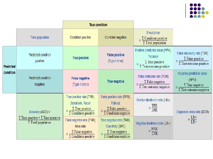
Example: confusion matrix • • • There were 214 data points. 47 of 51 input vectors that belonged to Class 1 and were correctly classified as Class 1. 162 of 163 input vectors that belonged to Class 2 and were correctly classified as Class 2.

Pattern Recognition Receiver Operating Characteristic (ROC) Curve l l l Receiver-operating characteristic (ROC) curves are an excellent way to compare diagnostic tests or pattern recognition. When we use the term Receiver Operating Characteristic or ROC curve, the receive we were originally talking about was a radar receiver in World War II. They were initially developed by the British. They were building the series of radar detectors to identify incoming German planes. But the radar detectors would also detect flocks of birds and other "false positive" signals. For example:

ROC Curve (continued) Radar detector setting Percent of geese German planes flocks correctly detected identified (sensitivity) (specificity) (true positive rate) (true negative rate) Percent of geese flocks incorrectly identified (1 - specificity) Off 0 100 0 Setting 1 35 93 7 Setting 2 60 85 15 Setting 3 Setting 4 Full 85 92 100 70 30 70 100 • As we turn the sensitivity of the receiver up, so it detects more and more German planes, it also mislabels more flocks of geese as Germany planes. • So, as sensitivity goes up, specificity goes down.

ROC Curve (continued) If we plot sensitivity against (1 – specificity) from the above table, here is what the graph looks like:

Pattern Recognition Receiver Operating Characteristic (ROC) Curve l l To create this curve, we take the output of the trained network and compare it against a threshold which ranges from -1 to +1 (assuming a tansig transfer function in the last layer). l Inputs that produce values above threshold are considered to belong to Class 1, and l those with values below the threshold are considered to belong to Class 2. l For each threshold value, we count the fraction of true positives and false positives in the data set. This pair of numbers produces one point on the ROC curve. As the threshold is varied, we trace the complete curve.

Receiver Operating Characteristic (ROC) Curve l The ideal point for the ROC curve to pass through would be (0, 1), which would correspond to no false positives and all true positives. l A poor ROC curve would represent a random guess, which is represented by the diagonal line passes through the point (0. 5, 0. 5).

ROC Curve (continued) l Since the diagonal line bisects the graph, the Area Under the ROC Curve (AUROCC) is 0. 5 for such a worthless test. l The best possible test (100% sensitive and 100% specific (would have an area under the curve of 1. 0 since the entire graph would fall beneath the curve. l While it is possible that the "perfectly bad test "would have an area of 0. 0, in reality we would just redefine what is positive and negative and it would become a perfect test.

ROC Curve (continued) l Thus, the AUROCC generally has a range of 0. 5 to 1. 0, with the following general interpretation: AUROCC Interpretation 1. 0 Perfect test 0. 9 to 0. 99 Excellent test 0. 8 to 0. 89 Good test 0. 7 to 0. 79 Fair test 0. 51 to 0. 69 Poor test 0. 5 Worthless test

Clustering (SOM) l Quantization Error: The average distance between each input vector and the closest prototype vector. l Topographic Error: The proportion of all input vectors for which the closest prototype vector and the next closest prototype vector are not neighbors in the feature map topology. l In a well trained SOM, prototypes that are neighbors in the topology should also be neighbors in the input space. l In this case, the topographic error should be zero.

Clustering (SOM) l 2 Distortion Measure: Where, hij is the neighborhood function, and cq is the index of the prototype that is closest to the input vector Pq, cq = arg minj{(||jw – pq||} Neighborhood function hij : • The simplest neighborhood function, is equal to 1 if prototype i is within some pre-specified neighborhood radius of prototype j, and equal to zero otherwise. • Other neighborhood functions possible is the Gaussian function where d is the neighborhood radius.

Prediction : Correlation of the prediction errors in time except at = 0 Inadequately Trained Network Successfully Trained Network Correlation in the prediction errors can indicate that the length of the tapped delay lines in the network should be increased.

Prediction: Correlation between the prediction errors and the input sequence Inadequately Trained Network Successfully Trained Network When using a NARX network, correlation between the prediction error and the input can suggest that the lengths of the tapped delay lines in the input and feedback paths should be increased.

Prediction Autocorrelation: l Correlation in the prediction errors in time Re( ) can indicate that the length of the tapped delay lines in the network should be increased. Cross Correlation: l When using a NARX network, correlation between the prediction error and the input Rpe( ) can suggest that the lengths of the tapped delay lines in the input and feedback paths should be increased.

Overfitting and Extrapolation If, after a network has been trained, the test set performance is not adequate, then there are usually four possible causes: l the network has reached a local minimum, l the network does not have enough neurons to fit the data, l the network is overfitting, or l the network is extrapolating.

Diagnosing Problems l l l The local minimum problem can almost always be overcome by retraining the network with five to ten random sets of initial weights. If the validation error is much larger than the training error, then overfitting has probably occurred. we can use a slower training algorithm to retrain the network If the validation, training and test errors are all similar in size, but the errors are too large, then the network is not powerful enough to fit the data. Add neurons. If the validation and training errors are similar in size, but the test errors are significantly larger, then the network may be extrapolating. If training, validation and test errors are similar, and the errors are small enough, then we can put the multilayer network to use.

Sensitivity Analysis: (importance of input vector elements) l l l After a multilayer network has been trained, it is often useful to assess the importance of each element of the input vector. If we can determine that a given element of the input vector is unimportant, then we can eliminate it. This can: l simplify the network, l reduce the amount of computation and l help prevent overfitting. There is no one method that can absolutely determine the importance of each input, but a sensitivity analysis can be helpful in this regard. A sensitivity analysis computes the derivatives of the network response with respect to each element of the input vector. If the derivative with respect to a certain input element is small, then that element can be eliminated from the input vector.

Sensitivity Analysis Check for important inputs

Sensitivity Analysis Remove unimportant inputs l l l This will be the derivative for a single squared error. To get the derivative of the sum square error, we sum the individual derivatives for each single squared error. The resulting vector will contain the derivatives of the sum square error for each element of the input vector. If we find that some of these derivatives are much smaller than the maximum derivative, then we can consider removing those inputs. Then retrain the network and compare the performance with the original network. If the performance is similar, then we accept the simplified network.