Practical Task Allocation for Software Fault Tolerance and




- Slides: 71

Practical Task Allocation for Software Fault Tolerance and Its Implementation in Embedded Automotive Systems Anand Bhat 1, Dr. Soheil Samii 2, Dr. Rajkumar 1 CMU 1 General Motors R&D 2 1

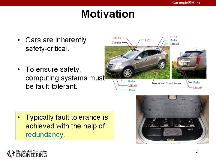
Motivation • Cars are inherently safety-critical. • To ensure safety, computing systems must be fault-tolerant. • Typically fault tolerance is achieved with the help of redundancy. 2

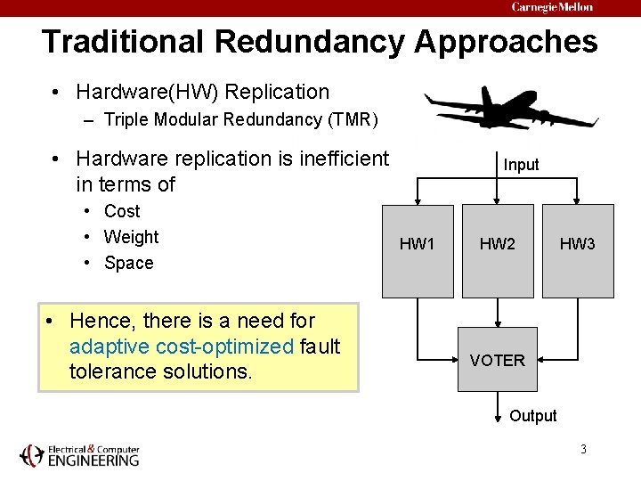
Traditional Redundancy Approaches • Hardware(HW) Replication – Triple Modular Redundancy (TMR) • Hardware replication is inefficient in terms of • Cost • Weight • Space • Hence, there is a need for adaptive cost-optimized fault tolerance solutions. Input HW 1 HW 2 HW 3 VOTER Output 3

Outline • System Model – Task Model – Platform Model • Fault Model • Fault-tolerant Task Allocation – TPCD Heuristic – TPCDC Heuristic – Evaluation • Software Fault Tolerance in Automotive Systems – Implementation – Evaluation • Conclusions 4

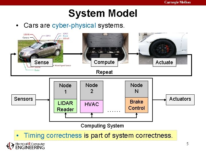
System Model • Cars are cyber-physical systems. Compute Sense Actuate Repeat Node 1 Sensors LIDAR Reader Node 2 Node N HVAC Brake Control …… Actuators Computing System • Timing correctness is part of system correctness. 5

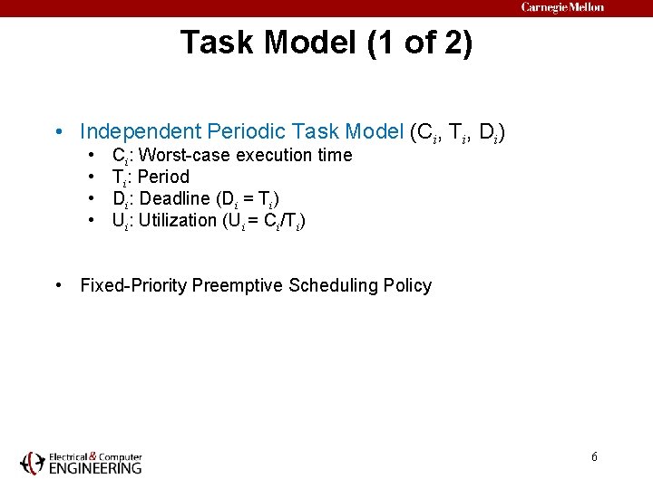
Task Model (1 of 2) • Independent Periodic Task Model (Ci, Ti, Di) • • Ci: Worst-case execution time Ti: Period Di: Deadline (Di = Ti) Ui: Utilization (Ui = Ci/Ti) • Fixed-Priority Preemptive Scheduling Policy 6

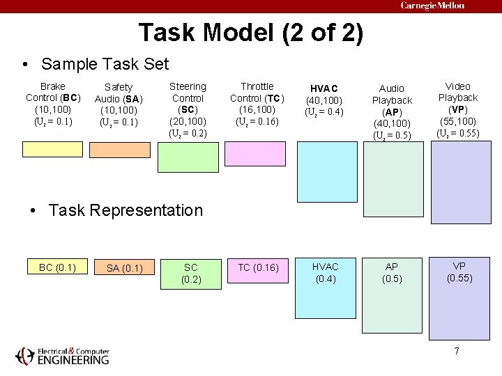
Task Model (2 of 2) • Sample Task Set Brake Control (BC) (10, 100) (Ui = 0. 1) Safety Audio (SA) (10, 100) (Ui = 0. 1) Steering Control (SC) (20, 100) (Ui = 0. 2) Throttle Control (TC) (16, 100) (Ui = 0. 16) HVAC (40, 100) (Ui = 0. 4) Audio Playback (AP) (40, 100) (Ui = 0. 5) Video Playback (VP) (55, 100) (Ui = 0. 55) TC (0. 16) HVAC (0. 4) AP (0. 5) VP (0. 55) • Task Representation BC (0. 1) SA (0. 1) SC (0. 2) 7

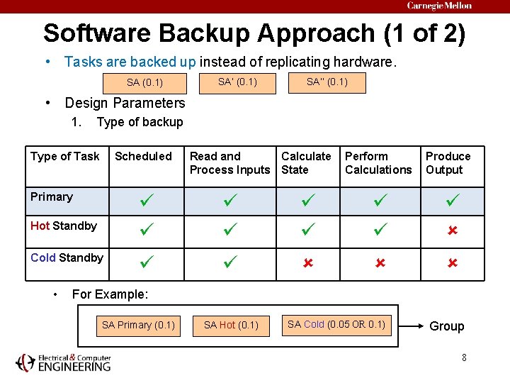
Software Backup Approach (1 of 2) • Tasks are backed up instead of replicating hardware. SA (0. 1) SA’’ (0. 1) • Design Parameters 1. Type of backup Type of Task Scheduled Primary Hot Standby Cold Standby • Read and Calculate Perform Process Inputs State Calculations Produce Output For Example: SA Primary (0. 1) SA Hot (0. 1) SA Cold (0. 05 OR 0. 1) Group 8

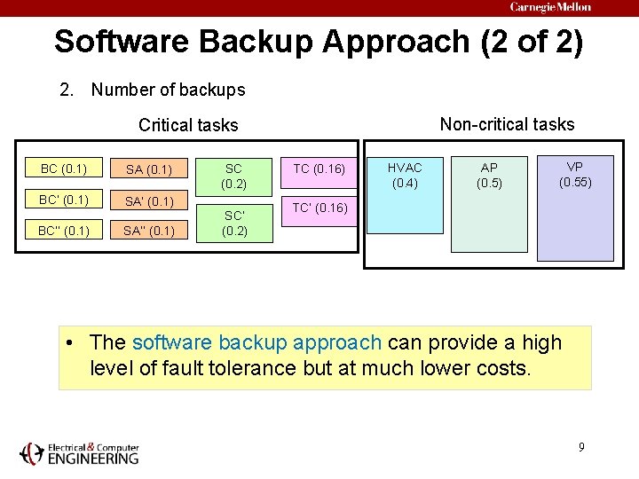
Software Backup Approach (2 of 2) 2. Number of backups Non-critical tasks Critical tasks BC (0. 1) SA (0. 1) BC’ (0. 1) SA’ (0. 1) BC’’ (0. 1) SA’’ (0. 1) SC (0. 2) SC’ (0. 2) TC (0. 16) HVAC (0. 4) AP (0. 5) VP (0. 55) TC’ (0. 16) • The software backup approach can provide a high level of fault tolerance but at much lower costs. 9

Outline • System Model – Task Model – Platform Model • Fault Model • The Fault-tolerant Task Allocation – TPCDC – Evaluation • Software Fault Tolerance Considerations in Automotive Systems – Implementation – Evaluation • Conclusions 10

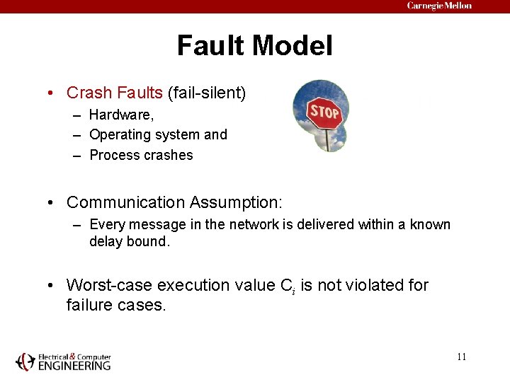
Fault Model • Crash Faults (fail-silent) – Hardware, – Operating system and – Process crashes • Communication Assumption: – Every message in the network is delivered within a known delay bound. • Worst-case execution value Ci is not violated for failure cases. 11

Outline • System Model – Task Model – Platform Model • Fault Model • The Fault-tolerant Task Allocation – TPCDC – Evaluation • Software Fault Tolerance Considerations in Automotive Systems – Implementation – Evaluation • Conclusions 12

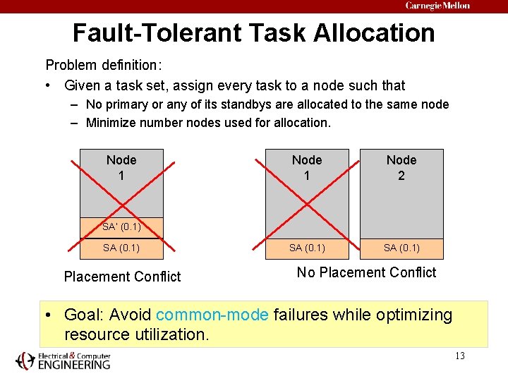
Fault-Tolerant Task Allocation Problem definition: • Given a task set, assign every task to a node such that – No primary or any of its standbys are allocated to the same node – Minimize number nodes used for allocation. Node 1 Node 2 SA (0. 1) SA’ (0. 1) SA (0. 1) Placement Conflict No Placement Conflict • Goal: Avoid common-mode failures while optimizing resource utilization. 13

Task Allocation Heuristics • Finding an optimal task allocation given an arbitrary task set is NP-hard. • Hence we use heuristics for task allocation. • Any Task Allocation Heuristic has 2 steps – Task Ordering – Node Ordering • We discuss 2 existing heuristics [14] – BFD-P – R-BFD 14

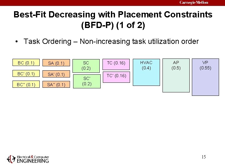
Best-Fit Decreasing with Placement Constraints (BFD-P) (1 of 2) • Task Ordering – Non-increasing task utilization order BC (0. 1) SA (0. 1) BC’ (0. 1) SA’ (0. 1) BC’’ (0. 1) SA’’ (0. 1) SC (0. 2) SC’ (0. 2) TC (0. 16) HVAC (0. 4) AP (0. 5) VP (0. 55) TC’ (0. 16) 15

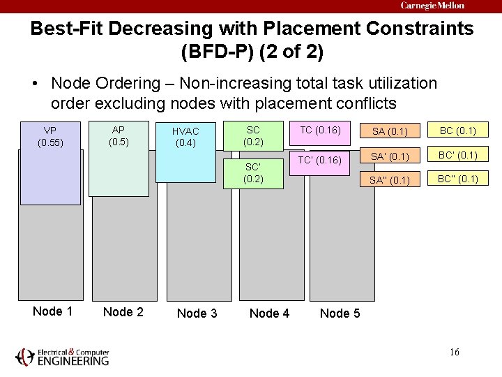
Best-Fit Decreasing with Placement Constraints (BFD-P) (2 of 2) • Node Ordering – Non-increasing total task utilization order excluding nodes with placement conflicts VP (0. 55) AP (0. 5) HVAC (0. 4) SC (0. 2) SC’ (0. 2) Node 1 Node 2 Node 3 Node 4 TC (0. 16) SA (0. 1) BC (0. 1) TC’ (0. 16) SA’ (0. 1) BC’ (0. 1) SA’’ (0. 1) BC’’ (0. 1) Node 5 16

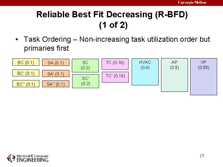
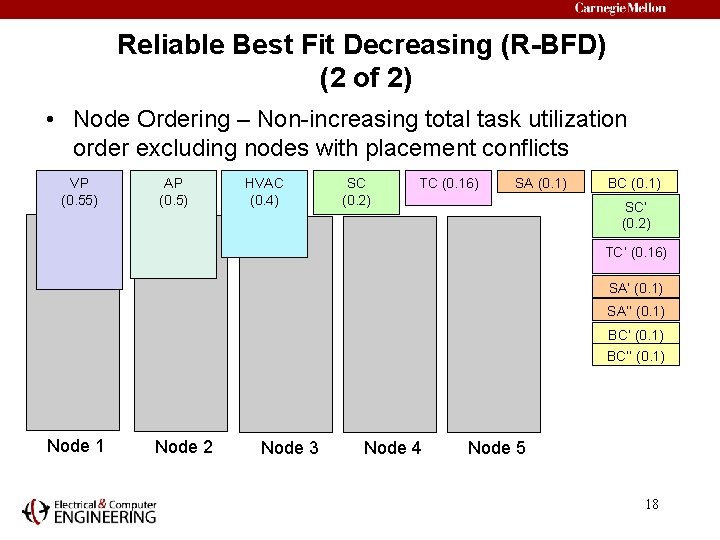
Reliable Best Fit Decreasing (R-BFD) (1 of 2) • Task Ordering – Non-increasing task utilization order but primaries first BC (0. 1) SA (0. 1) BC’ (0. 1) SA’ (0. 1) BC’’ (0. 1) SA’’ (0. 1) SC (0. 2) SC’ (0. 2) TC (0. 16) HVAC (0. 4) AP (0. 5) VP (0. 55) TC’ (0. 16) 17

Reliable Best Fit Decreasing (R-BFD) (2 of 2) • Node Ordering – Non-increasing total task utilization order excluding nodes with placement conflicts VP (0. 55) AP (0. 5) HVAC (0. 4) SC (0. 2) TC (0. 16) SA (0. 1) BC (0. 1) SC’ (0. 2) TC’ (0. 16) SA’ (0. 1) SA’’ (0. 1) BC’’ (0. 1) Node 1 Node 2 Node 3 Node 4 Node 5 18

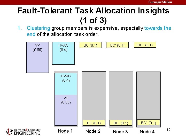
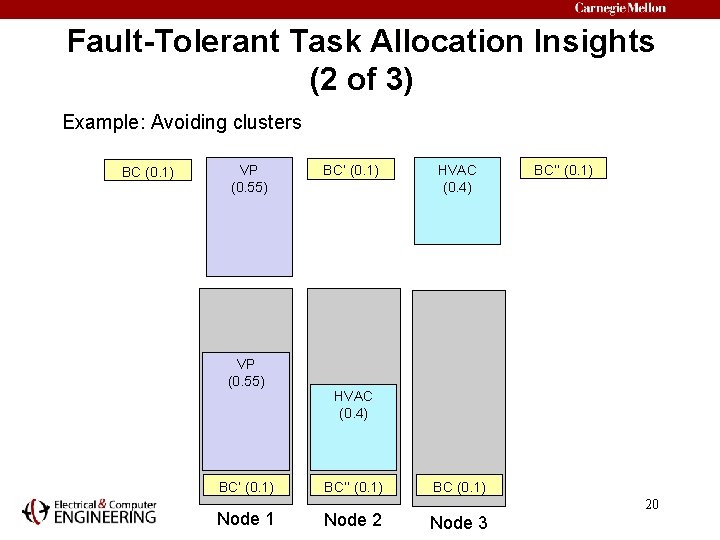
Fault-Tolerant Task Allocation Insights (1 of 3) 1. Clustering group members is expensive, especially towards the end of the allocation task order. VP (0. 55) HVAC (0. 4) BC (0. 1) BC’’ (0. 1) HVAC (0. 4) VP (0. 55) Node 1 BC (0. 1) BC’ (0. 1) Node 2 Node 3 BC’’ (0. 1) Node 4 19

Fault-Tolerant Task Allocation Insights (2 of 3) Example: Avoiding clusters BC (0. 1) VP (0. 55) BC’ (0. 1) Node 1 BC’ (0. 1) HVAC (0. 4) BC’’ (0. 1) Node 2 BC (0. 1) 20 Node 3

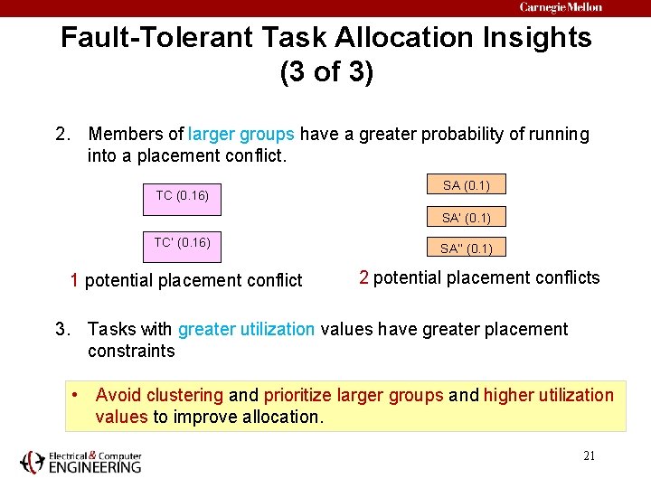
Fault-Tolerant Task Allocation Insights (3 of 3) 2. Members of larger groups have a greater probability of running into a placement conflict. TC (0. 16) SA (0. 1) SA’ (0. 1) TC’ (0. 16) 1 potential placement conflict SA’’ (0. 1) 2 potential placement conflicts 3. Tasks with greater utilization values have greater placement constraints • Avoid clustering and prioritize larger groups and higher utilization values to improve allocation. 21

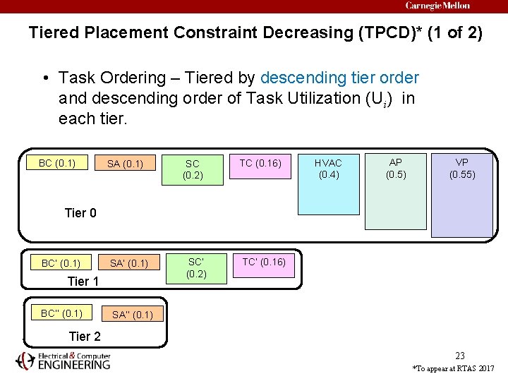
Tiered Placement Constraint Decreasing (TPCD)* (1 of 2) • Task Ordering – Tiered by descending tier order and descending order of Task Utilization (Ui) in each tier. BC (0. 1) SA (0. 1) SC (0. 2) TC (0. 16) HVAC (0. 4) AP (0. 5) VP (0. 55) Tier 0 BC’ (0. 1) SA’ (0. 1) Tier 1 BC’’ (0. 1) SC’ (0. 2) TC’ (0. 16) SA’’ (0. 1) Tier 2 22 *To appear at RTAS 2017

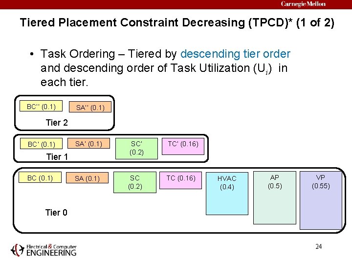
Tiered Placement Constraint Decreasing (TPCD)* (1 of 2) • Task Ordering – Tiered by descending tier order and descending order of Task Utilization (Ui) in each tier. BC (0. 1) SA (0. 1) SC (0. 2) TC (0. 16) HVAC (0. 4) AP (0. 5) VP (0. 55) Tier 0 BC’ (0. 1) SA’ (0. 1) Tier 1 BC’’ (0. 1) SC’ (0. 2) TC’ (0. 16) SA’’ (0. 1) Tier 2 23 *To appear at RTAS 2017

Tiered Placement Constraint Decreasing (TPCD)* (1 of 2) • Task Ordering – Tiered by descending tier order and descending order of Task Utilization (Ui) in each tier. BC’’ (0. 1) SA’’ (0. 1) Tier 2 BC’ (0. 1) SA’ (0. 1) SC’ (0. 2) TC’ (0. 16) SA (0. 1) SC (0. 2) TC (0. 16) Tier 1 BC (0. 1) HVAC (0. 4) AP (0. 5) VP (0. 55) Tier 0 24

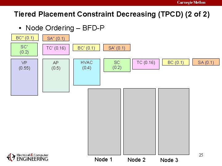
Tiered Placement Constraint Decreasing (TPCD) (2 of 2) • Node Ordering – BFD-P BC’’ (0. 1) SA’’ (0. 1) SC’ (0. 2) TC’ (0. 16) BC’ (0. 1) SA’ (0. 1) VP (0. 55) AP (0. 5) HVAC (0. 4) SC (0. 2) Node 1 TC (0. 16) Node 2 BC (0. 1) Node 3 SA (0. 1) 25

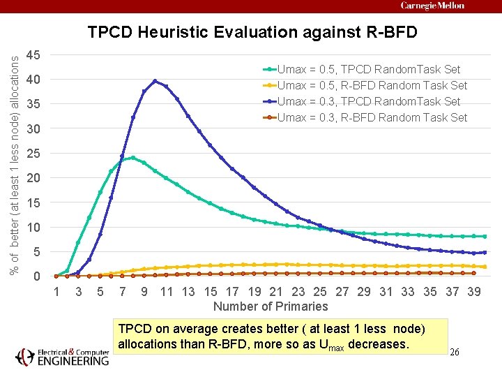
% of better (at least 1 less node) allocations TPCD Heuristic Evaluation against R-BFD 45 Umax = 0. 5, TPCD Random. Task Set Umax = 0. 5, R-BFD Random Task Set Umax = 0. 3, TPCD Random. Task Set Umax = 0. 3, R-BFD Random Task Set 40 35 30 25 20 15 10 5 0 1 3 5 7 9 11 13 15 17 19 21 23 25 27 29 31 33 35 37 39 Number of Primaries TPCD on average creates better ( at least 1 less node) allocations than R-BFD, more so as Umax decreases. 26

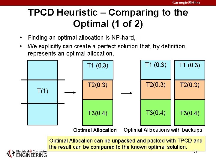
TPCD Heuristic – Comparing to the Optimal (1 of 2) • Finding an optimal allocation is NP-hard, • We explicitly can create a perfect solution that, by definition, represents an optimal allocation. T(1) T 1 (0. 3) T 2(0. 3) 0. 4 T 3(0. 4) Optimal Allocations with backups Optimal Allocation can be unpacked and packed with TPCD and the result can be compared to the known optimal solution. 27

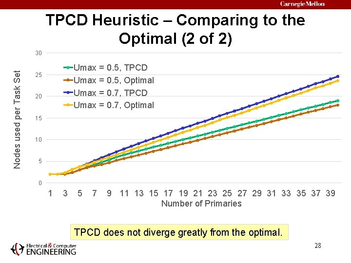
TPCD Heuristic – Comparing to the Optimal (2 of 2) Nodes used per Task Set 30 Umax = 0. 5, TPCD Umax = 0. 5, Optimal Umax = 0. 7, TPCD Umax = 0. 7, Optimal 25 20 15 10 5 0 1 3 5 7 9 11 13 15 17 19 21 23 25 27 29 31 33 35 37 39 Number of Primaries TPCD does not diverge greatly from the optimal. 28

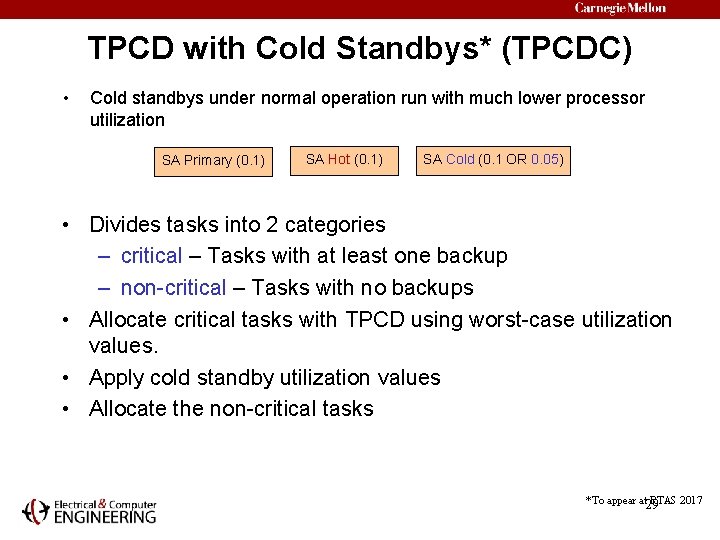
TPCD with Cold Standbys* (TPCDC) • Cold standbys under normal operation run with much lower processor utilization SA Primary (0. 1) SA Hot (0. 1) SA Cold (0. 1 OR 0. 05) • Divides tasks into 2 categories – critical – Tasks with at least one backup – non-critical – Tasks with no backups • Allocate critical tasks with TPCD using worst-case utilization values. • Apply cold standby utilization values • Allocate the non-critical tasks *To appear at 29 RTAS 2017

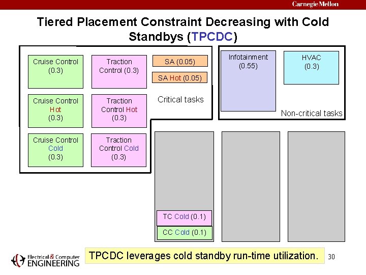
Tiered Placement Constraint Decreasing with Cold Standbys (TPCDC) Cruise Control (0. 3) Traction Control (0. 3) Cruise Control Hot (0. 3) Traction Control Hot (0. 3) Cruise Control Cold (0. 3) Traction Control Cold (0. 3) SA (0. 05) Infotainment (0. 55) HVAC (0. 3) SA Hot (0. 05) Critical tasks Non-critical tasks TC Cold (0. 1) CC Cold (0. 1) TPCDC leverages cold standby run-time utilization. 30

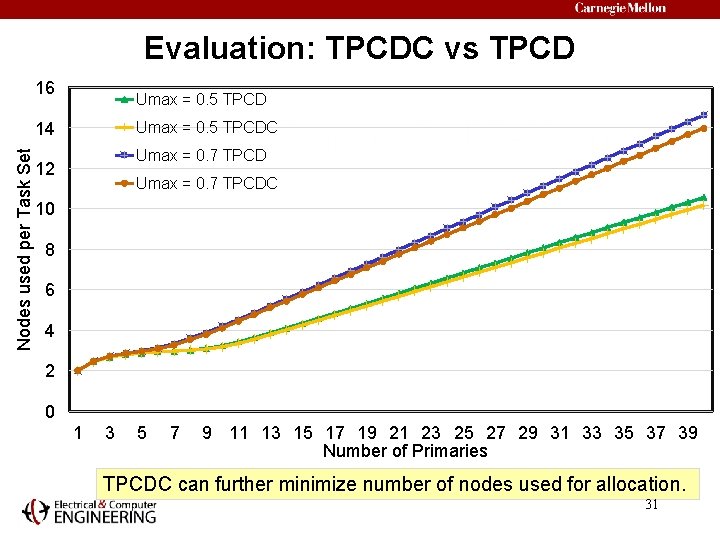
Evaluation: TPCDC vs TPCD 16 Umax = 0. 5 TPCD Nodes used per Task Set 14 Umax = 0. 5 TPCDC Umax = 0. 7 TPCD 12 Umax = 0. 7 TPCDC 10 8 6 4 2 0 1 3 5 7 9 11 13 15 17 19 21 23 25 27 29 31 33 35 37 39 Number of Primaries TPCDC can further minimize number of nodes used for allocation. 31

Outline • System Model – Task Model – Platform Model • Fault Model • The Fault-tolerant Task Allocation – TPCDC – Evaluation • Software Fault Tolerance Considerations in Automotive Systems – Implementation – Evaluation • Conclusions 32

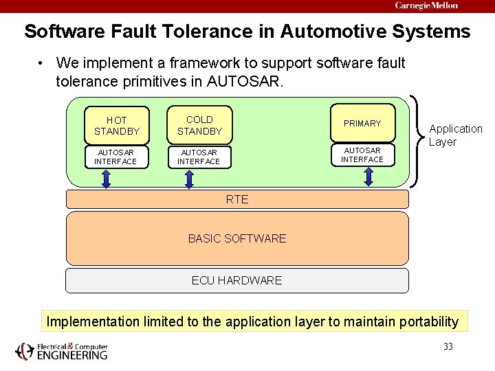
Software Fault Tolerance in Automotive Systems • We implement a framework to support software fault tolerance primitives in AUTOSAR. HOT STANDBY COLD STANDBY PRIMARY AUTOSAR INTERFACE Application Layer RTE BASIC SOFTWARE ECU HARDWARE Implementation limited to the application layer to maintain portability 33

Features of our Software Fault Tolerance Framework • Standby Creation and Configuration • Support for Group Formation and Maintenance • Supports Failure Recovery • Supports Dynamic Reconfiguration 34

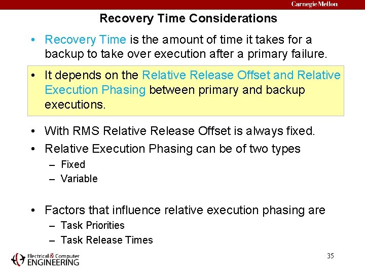
Recovery Time Considerations • Recovery Time is the amount of time it takes for a backup to take over execution after a primary failure. • It depends on the Relative Release Offset and Relative Execution Phasing between primary and backup executions. • With RMS Relative Release Offset is always fixed. • Relative Execution Phasing can be of two types – Fixed – Variable • Factors that influence relative execution phasing are – Task Priorities – Task Release Times 35

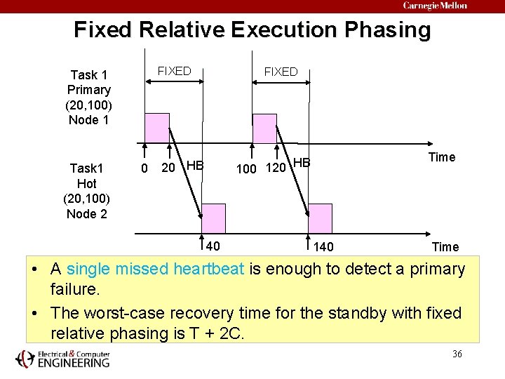
Fixed Relative Execution Phasing FIXED Task 1 Primary (20, 100) Node 1 Task 1 Hot (20, 100) Node 2 0 FIXED Time 100 120 HB 40 140 Time • A single missed heartbeat is enough to detect a primary failure. • The worst-case recovery time for the standby with fixed relative phasing is T + 2 C. 36

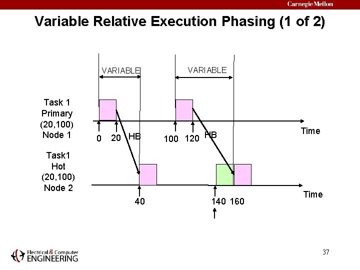
Variable Relative Execution Phasing (1 of 2) VARIABLE Task 1 Primary (20, 100) Node 1 0 20 HB VARIABLE 100 120 HB Task 1 Hot (20, 100) Node 2 40 160 Time 37

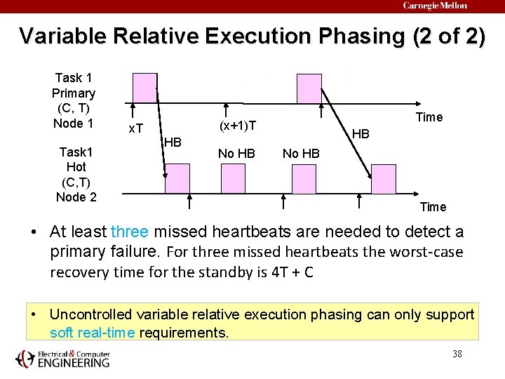
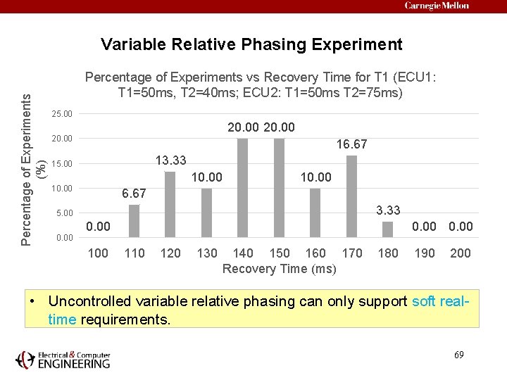
Variable Relative Execution Phasing (2 of 2) Task 1 Primary (C, T) Node 1 Task 1 Hot (C, T) Node 2 Time (x+1)T x. T HB No HB Time • At least three missed heartbeats are needed to detect a primary failure. For three missed heartbeats the worst-case recovery time for the standby is 4 T + C • Uncontrolled variable relative execution phasing can only support soft real-time requirements. 38

Future Directions • Recovery Time for Variable Relative Execution Phasing can be improved by controlling relative release offsets. • Such phase control can allow hard real-time guarantees even without fixed relative execution phasing. • Standby type assignment and task allocation can be decided to guarantee application recovery time requirements. 39

Conclusions • The Fault-tolerant task allocation problem addresses common mode failures while reducing resource utilization. – The TPCD heuristic on average produces a better allocation than R-BFD. – The TPCDC heuristic leverages the run-time characteristics of cold standbys, further improving the resource utilization compared to TPCD. • The software backup approach can be adapted for the automotive context in order to achieve dependable operation with the help of phase control. 40

Thank you 41

Questions? 42

Backup Slides 43

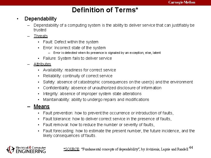
Definition of Terms* • Dependability – Dependability of a computing system is the ability to deliver service that can justifiably be trusted – Threats • Fault: Defect within the system • Error: Incorrect state of the system – Error is detected when its presence is signaled by an exception; else, latent • Failure: System fails to deliver service – Attributes • Availability: readiness for correct service • Reliability: continuity of correct service • Safety: absence of catastrophic consequences on the user(s) and the environment • Confidentiality: absence of unauthorized disclosure of information • Integrity: absence of improper system state alterations • Maintainability: ability to undergo repairs and modifications – Means • • Fault prevention: how to prevent the occurrence or introduction of faults, Fault tolerance: how to deliver correct service in the presence of faults, Fault removal: how to reduce the number or severity of faults, Fault forecasting: how to estimate the present number, the future incidence, and the likely consequences of faults. *SOURCE: “Fundamental concepts of dependability”, by Avizienis, Laprie and Randell 44

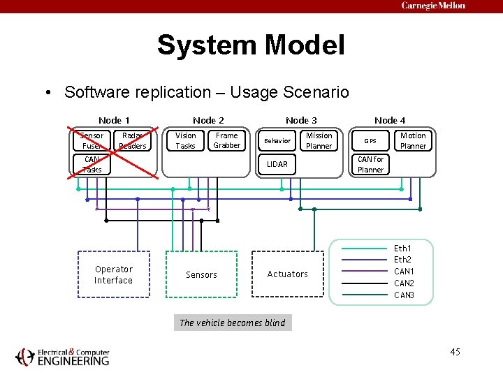
System Model • Software replication – Usage Scenario Node 1 Sensor Fuser Radar Readers Node 2 Vision Tasks Frame Grabber CAN Tasks Operator Interface Node 3 Behavior Mission Planner LIDAR Sensors Actuators Node 4 GPS Motion Planner CAN for Planner Eth 1 Eth 2 CAN 1 CAN 2 CAN 3 The vehicle becomes blind 45

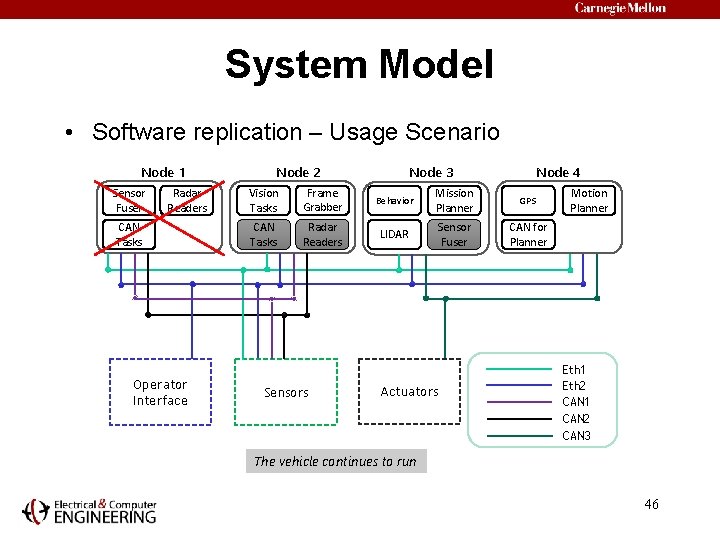
System Model • Software replication – Usage Scenario Node 1 Sensor Fuser Radar Readers CAN Tasks Operator Interface Node 2 Node 3 Node 4 Vision Tasks Frame Grabber Behavior Mission Planner GPS CAN Tasks Radar Readers LIDAR Sensor Fuser CAN for Planner Sensors Actuators Motion Planner Eth 1 Eth 2 CAN 1 CAN 2 CAN 3 The vehicle continues to run 46

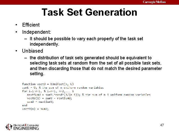
Task Set Generation • Efficient • Independent: – It should be possible to vary each property of the task set independently. • Unbiased – the distribution of task sets generated should be equivalent to selecting task sets at random from the set of all possible task sets, and then discarding those that do not match the desired parameter setting. 47

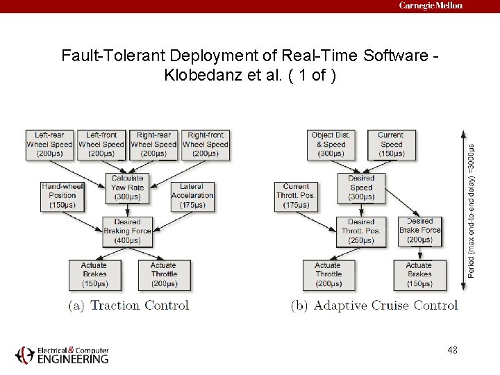
Fault-Tolerant Deployment of Real-Time Software Klobedanz et al. ( 1 of ) 48

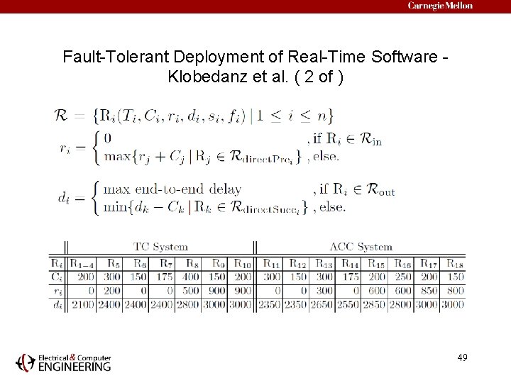
Fault-Tolerant Deployment of Real-Time Software Klobedanz et al. ( 2 of ) 49

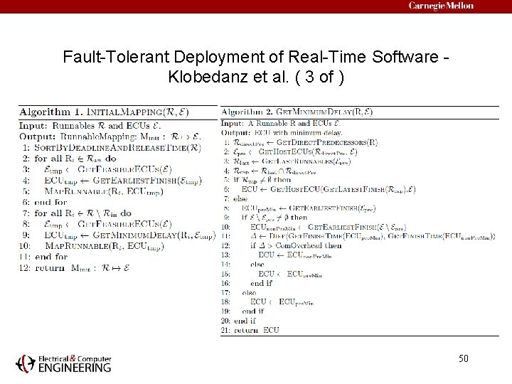
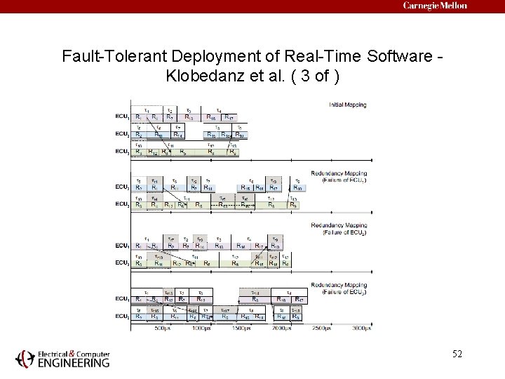
Fault-Tolerant Deployment of Real-Time Software Klobedanz et al. ( 3 of ) 50

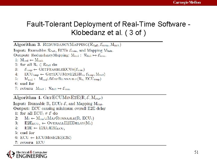
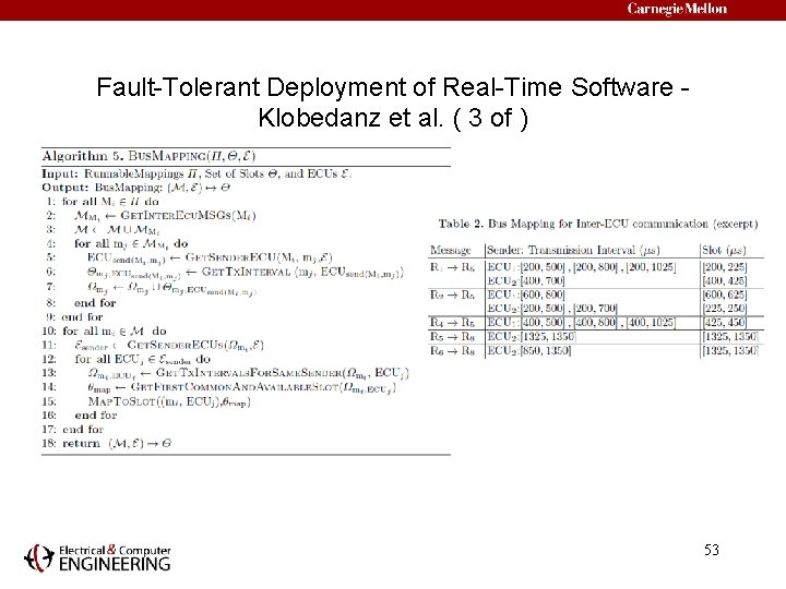
Fault-Tolerant Deployment of Real-Time Software Klobedanz et al. ( 3 of ) 51

Fault-Tolerant Deployment of Real-Time Software Klobedanz et al. ( 3 of ) 52

Fault-Tolerant Deployment of Real-Time Software Klobedanz et al. ( 3 of ) 53

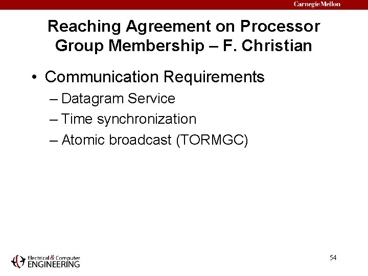
Reaching Agreement on Processor Group Membership – F. Christian • Communication Requirements – Datagram Service – Time synchronization – Atomic broadcast (TORMGC) 54

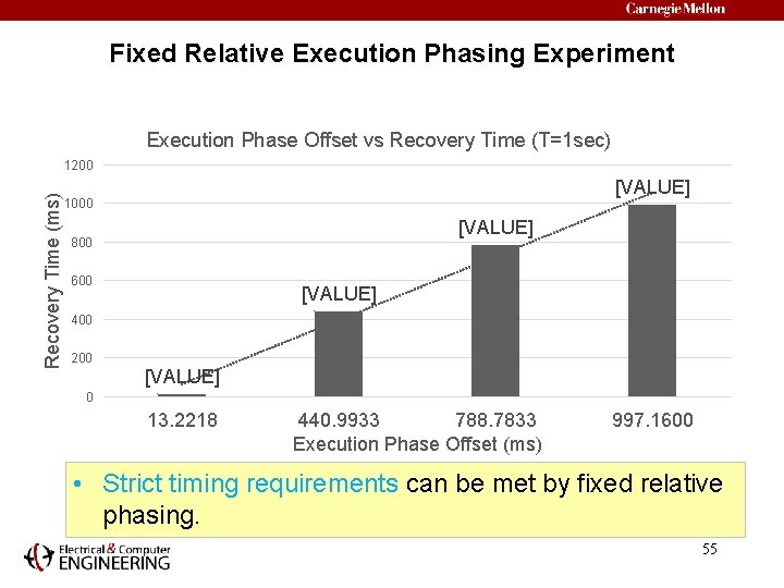
Fixed Relative Execution Phasing Experiment Execution Phase Offset vs Recovery Time (T=1 sec) Recovery Time (ms) 1200 [VALUE] 1000 [VALUE] 800 600 [VALUE] 400 200 [VALUE] 0 13. 2218 440. 9933 788. 7833 Execution Phase Offset (ms) 997. 1600 • Strict timing requirements can be met by fixed relative phasing. 55

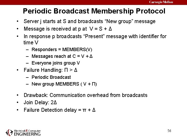
Periodic Broadcast Membership Protocol • Server j starts at S and broadcasts “New group” message • Message is received at p at V = S + Δ • In response p broadcasts “Present” message with identifier for time V – Responders = MEMBERS(V) – Messages reach at C = V + Δ – Everyone joins group V • Failure Handling: Π > Δ – Periodic Broadcast – New group MEMBERS ( V + Π) • Drawback: Communication overhead from broadcasts • Join Delay: 2Δ • Failure Detection delay = π + Δ 56

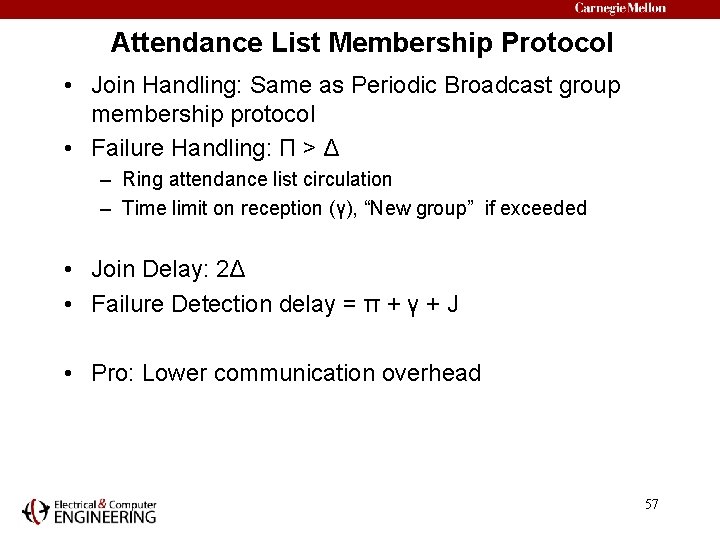
Attendance List Membership Protocol • Join Handling: Same as Periodic Broadcast group membership protocol • Failure Handling: Π > Δ – Ring attendance list circulation – Time limit on reception (γ), “New group” if exceeded • Join Delay: 2Δ • Failure Detection delay = π + γ + J • Pro: Lower communication overhead 57

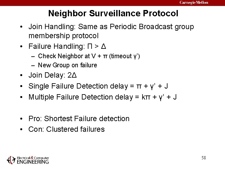
Neighbor Surveillance Protocol • Join Handling: Same as Periodic Broadcast group membership protocol • Failure Handling: Π > Δ – Check Neighbor at V + π (timeout γ’) – New Group on failure • Join Delay: 2Δ • Single Failure Detection delay = π + γ’ + J • Multiple Failure Detection delay = kπ + γ’ + J • Pro: Shortest Failure detection • Con: Clustered failures 58

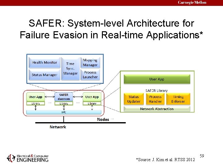
SAFER: System-level Architecture for Failure Evasion in Real-time Applications* *Source: J. Kim et al. RTSS 2012 59

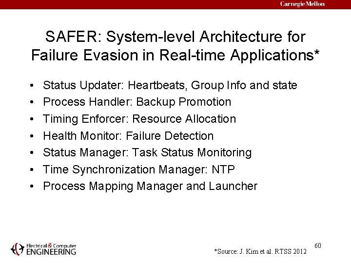
SAFER: System-level Architecture for Failure Evasion in Real-time Applications* • • Status Updater: Heartbeats, Group Info and state Process Handler: Backup Promotion Timing Enforcer: Resource Allocation Health Monitor: Failure Detection Status Manager: Task Status Monitoring Time Synchronization Manager: NTP Process Mapping Manager and Launcher *Source: J. Kim et al. RTSS 2012 60

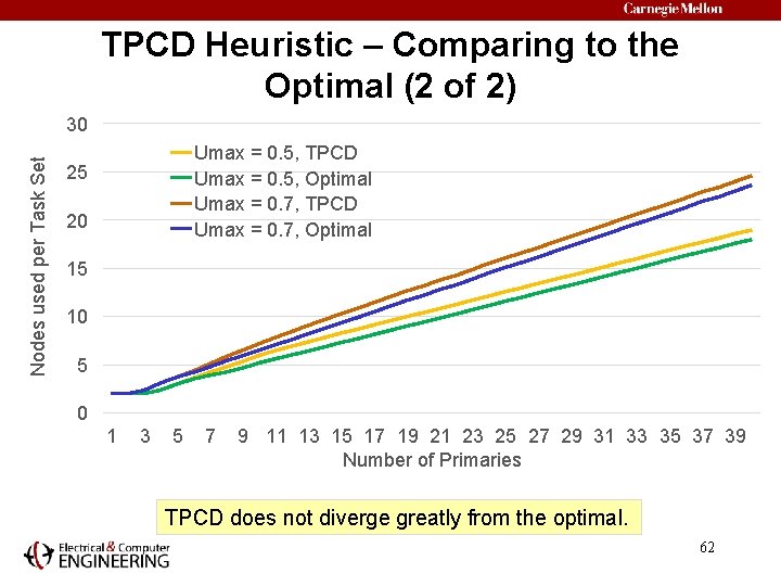
TPCD Heuristic – Comparing to the Optimal (1 of 2) • Finding an optimal allocation is NP-hard, • We explicitly can create a perfect solution that, by definition, represents an optimal allocation. T(1) T 1 (0. 3) T 2(0. 3) 0. 4 T 3(0. 4) Optimal Allocations with backups Optimal Allocation can be unpacked and packed with TPCD and the result can be compared to the known optimal solution. 61

TPCD Heuristic – Comparing to the Optimal (2 of 2) Nodes used per Task Set 30 Umax = 0. 5, TPCD Umax = 0. 5, Optimal Umax = 0. 7, TPCD Umax = 0. 7, Optimal 25 20 15 10 5 0 1 3 5 7 9 11 13 15 17 19 21 23 25 27 29 31 33 35 37 39 Number of Primaries TPCD does not diverge greatly from the optimal. 62

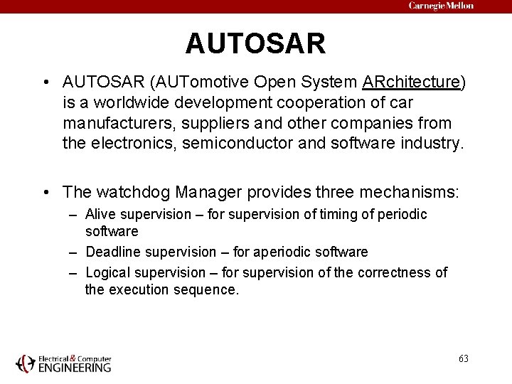
AUTOSAR • AUTOSAR (AUTomotive Open System ARchitecture) is a worldwide development cooperation of car manufacturers, suppliers and other companies from the electronics, semiconductor and software industry. • The watchdog Manager provides three mechanisms: – Alive supervision – for supervision of timing of periodic software – Deadline supervision – for aperiodic software – Logical supervision – for supervision of the correctness of the execution sequence. 63

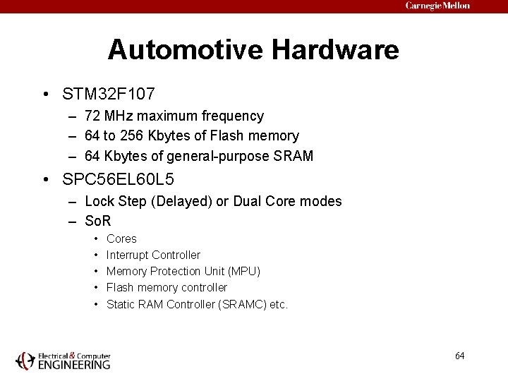
Automotive Hardware • STM 32 F 107 – 72 MHz maximum frequency – 64 to 256 Kbytes of Flash memory – 64 Kbytes of general-purpose SRAM • SPC 56 EL 60 L 5 – Lock Step (Delayed) or Dual Core modes – So. R • • • Cores Interrupt Controller Memory Protection Unit (MPU) Flash memory controller Static RAM Controller (SRAMC) etc. 64

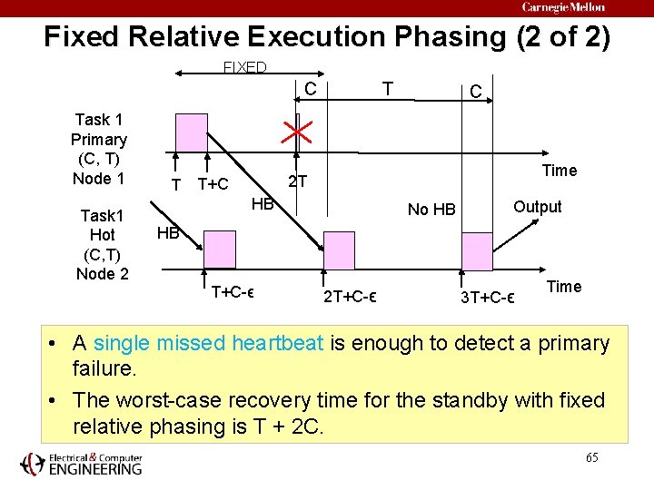
Fixed Relative Execution Phasing (2 of 2) FIXED T C Task 1 Primary (C, T) Node 1 Task 1 Hot (C, T) Node 2 C Time 2 T T T+C HB No HB Output HB T+C-ϵ 2 T+C-ϵ 3 T+C-ϵ Time • A single missed heartbeat is enough to detect a primary failure. • The worst-case recovery time for the standby with fixed relative phasing is T + 2 C. 65

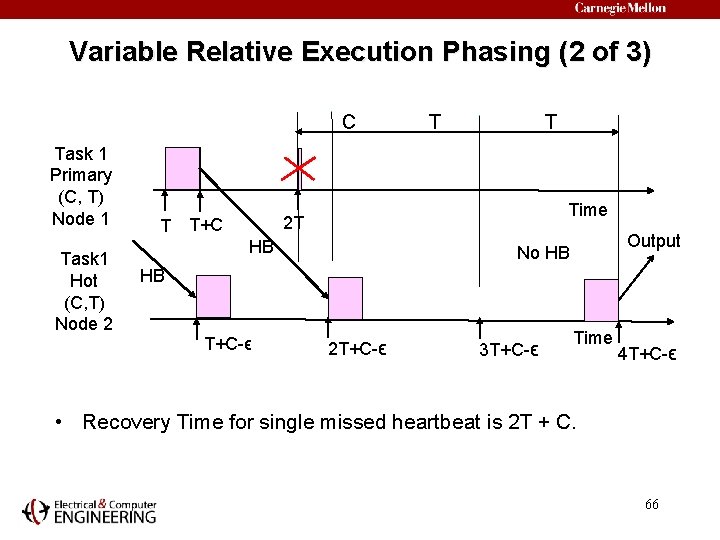
Variable Relative Execution Phasing (2 of 3) C Task 1 Primary (C, T) Node 1 Task 1 Hot (C, T) Node 2 T T Time 2 T T T+C HB Output No HB HB T+C-ϵ 2 T+C-ϵ 3 T+C-ϵ Time 4 T+C-ϵ • Recovery Time for single missed heartbeat is 2 T + C. 66

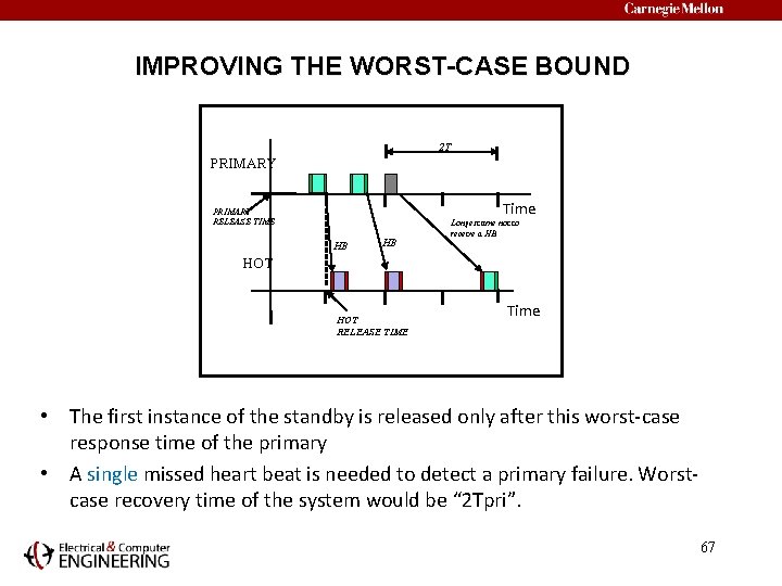
IMPROVING THE WORST-CASE BOUND 2 T PRIMARY Time PRIMARY RELEASE TIME HB HB Longest time not to receive a HB HOT RELEASE TIME Time • The first instance of the standby is released only after this worst-case response time of the primary • A single missed heart beat is needed to detect a primary failure. Worstcase recovery time of the system would be “ 2 Tpri”. 67

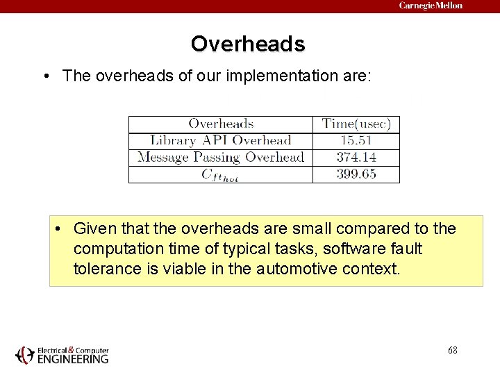
Overheads • The overheads of our implementation are: • Given that the overheads are small compared to the computation time of typical tasks, software fault tolerance is viable in the automotive context. 68

Percentage of Experiments (%) Variable Relative Phasing Experiment Percentage of Experiments vs Recovery Time for T 1 (ECU 1: T 1=50 ms, T 2=40 ms; ECU 2: T 1=50 ms T 2=75 ms) 25. 00 20. 00 16. 67 13. 33 15. 00 10. 00 6. 67 3. 33 5. 00 0. 00 100 0. 00 110 120 130 140 150 160 170 Recovery Time (ms) 180 190 200 • Uncontrolled variable relative phasing can only support soft realtime requirements. 69

70 Source: SAE

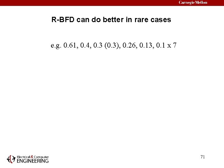
R-BFD can do better in rare cases e. g. 0. 61, 0. 4, 0. 3 (0. 3), 0. 26, 0. 13, 0. 1 x 7 71