Practical Radio Propagation Models Radio Propagation Models T

Practical Radio Propagation Models

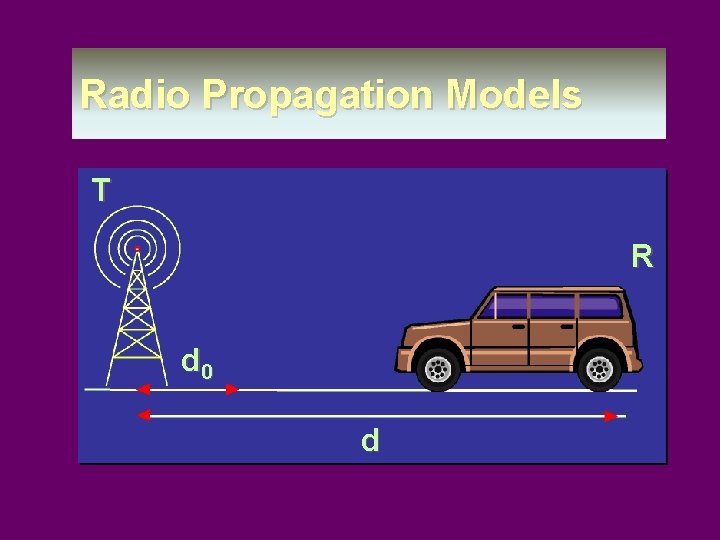
Radio Propagation Models T R d 0 d

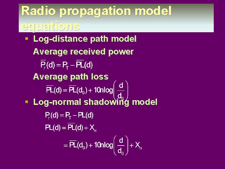
Radio propagation model equations § Log-distance path model Average received power Average path loss § Log-normal shadowing model

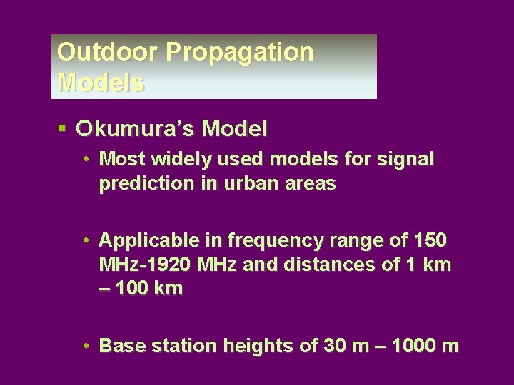
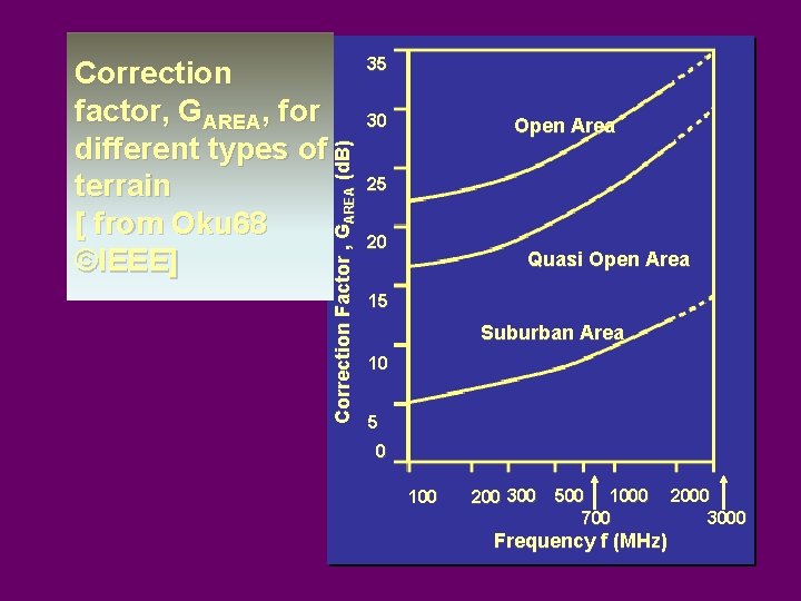
Outdoor Propagation Models § Okumura’s Model • Most widely used models for signal prediction in urban areas • Applicable in frequency range of 150 MHz-1920 MHz and distances of 1 km – 100 km • Base station heights of 30 m – 1000 m

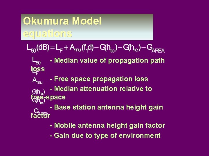
Okumura Model equations - Median value of propagation path loss - Free space propagation loss - Median attenuation relative to free-space - Base station antenna height gain factor - Mobile antenna height gain factor - Gain due to type of environment

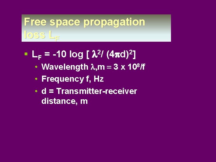
Free space propagation loss LF § LF = -10 log [ l 2/ (4 pd)2] • • • Wavelength l, m = 3 x 108/f Frequency f, Hz d = Transmitter-receiver distance, m

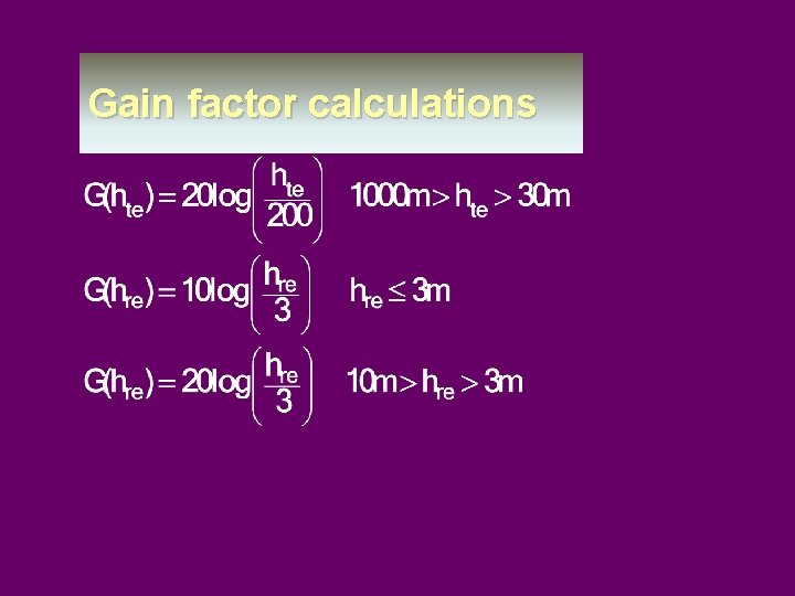
Gain factor calculations

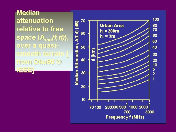
100 70 Urban Area ht = 200 m hr = 3 m 60 50 40 d (km) Median Attenuation, A(f, d) (d. B) Median attenuation relative to free space (Amu(f, d)), over a quasismooth terrain [ from Oku 68 © IEEE] 80 70 60 50 40 30 20 10 5 2 1 30 20 10 70 100 200300 500 1000 2000 3000 700 Frequency f (MHz)

Correction Factor , GAREA (d. B) Correction factor, GAREA, for different types of terrain [ from Oku 68 ©IEEE] 35 30 Open Area 25 20 Quasi Open Area 15 Suburban Area 10 5 0 100 200 300 500 1000 700 Frequency f (MHz) 2000 3000

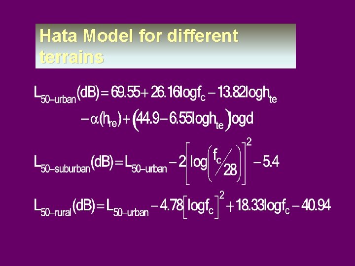
Hata Model for different terrains |

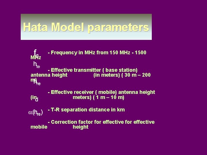
Hata Model parameters - Frequency in MHz from 150 MHz - 1500 MHz - Effective transmitter ( base station) antenna height (in meters) ( 30 m – 200 m) - Effective receiver ( mobile) antenna height (in meters) ( 1 m – 10 m) - T-R separation distance in km - Correction factor for effective mobile height

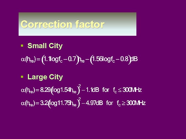
Correction factor § Small City § Large City

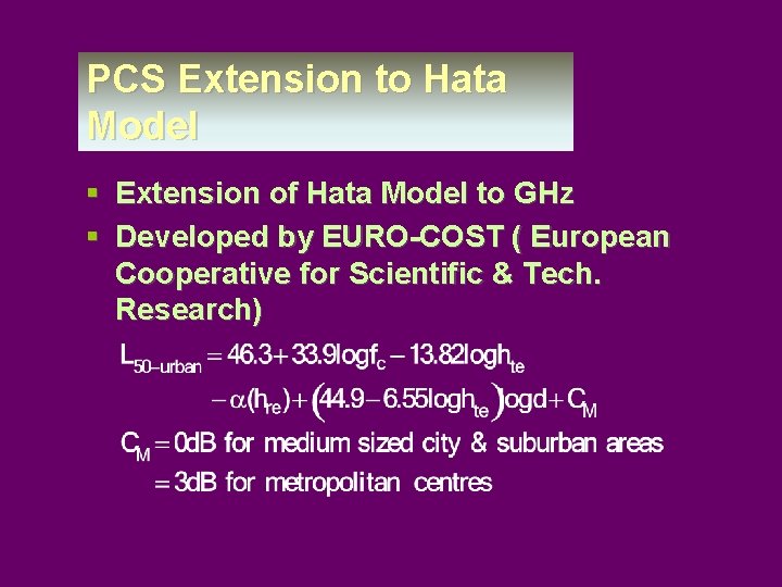
PCS Extension to Hata Model § Extension of Hata Model to GHz § Developed by EURO-COST ( European Cooperative for Scientific & Tech. Research)

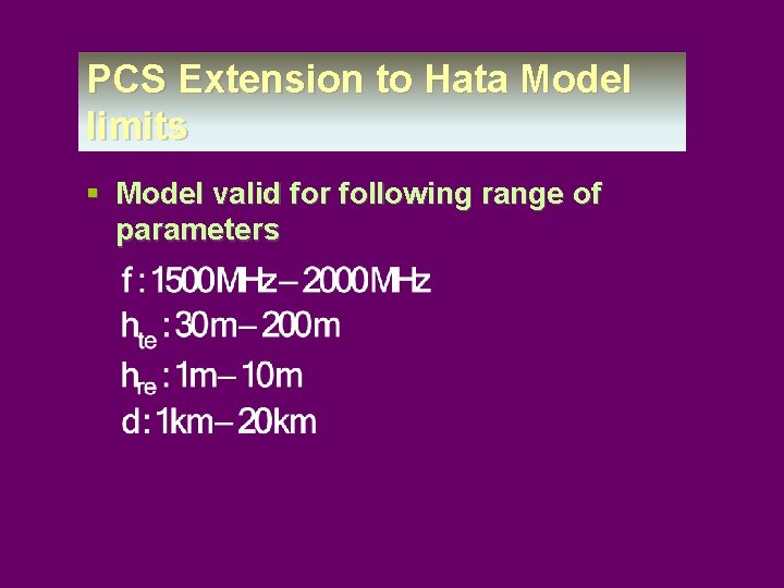
PCS Extension to Hata Model limits § Model valid for following range of parameters

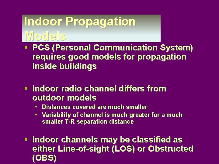
Indoor Propagation Models § PCS (Personal Communication System) requires good models for propagation inside buildings § Indoor radio channel differs from outdoor models • Distances covered are much smaller • Variability of channel is much greater for a much smaller T-R separation distance § Indoor channels may be classified as either Line-of-sight (LOS) or Obstructed (OBS)

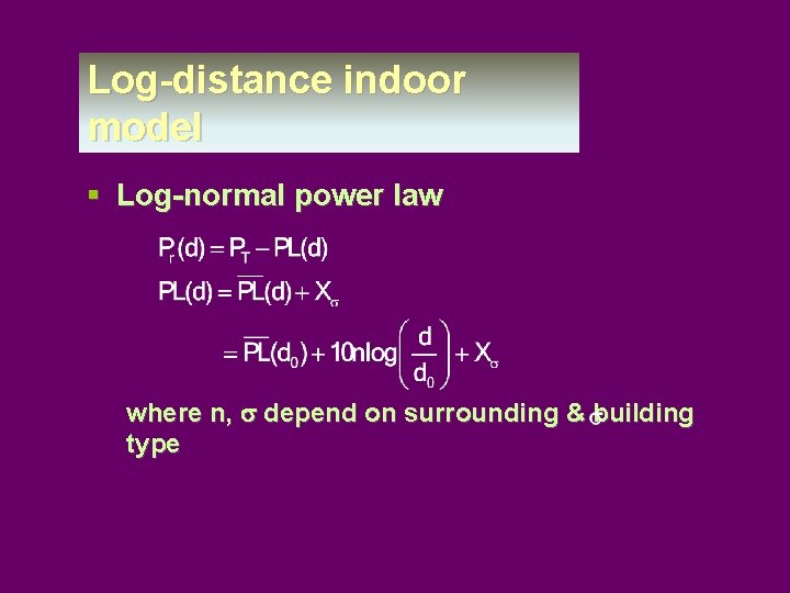
Log-distance indoor model § Log-normal power law where n, s depend on surrounding & building type

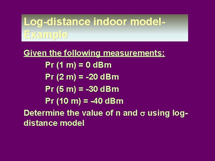
Log-distance indoor model- Example Given the following measurements: Pr (1 m) = 0 d. Bm Pr (2 m) = -20 d. Bm Pr (5 m) = -30 d. Bm Pr (10 m) = -40 d. Bm Determine the value of n and s using logdistance model

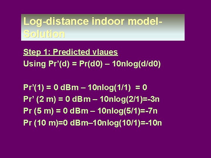
Log-distance indoor model- Solution Step 1: Predicted vlaues Using Pr’(d) = Pr(d 0) – 10 nlog(d/d 0) Pr’(1) = 0 d. Bm – 10 nlog(1/1) = 0 Pr’ (2 m) = 0 d. Bm – 10 nlog(2/1)=-3 n Pr (5 m) = 0 d. Bm – 10 nlog(5/1)=-7 n Pr (10 m)=0 d. Bm– 10 nlog(10/1)=-10 n

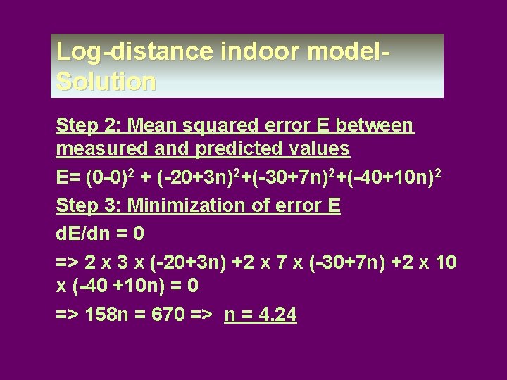
Log-distance indoor model- Solution Step 2: Mean squared error E between measured and predicted values E= (0 -0)2 + (-20+3 n)2+(-30+7 n)2+(-40+10 n)2 Step 3: Minimization of error E d. E/dn = 0 => 2 x 3 x (-20+3 n) +2 x 7 x (-30+7 n) +2 x 10 x (-40 +10 n) = 0 => 158 n = 670 => n = 4. 24

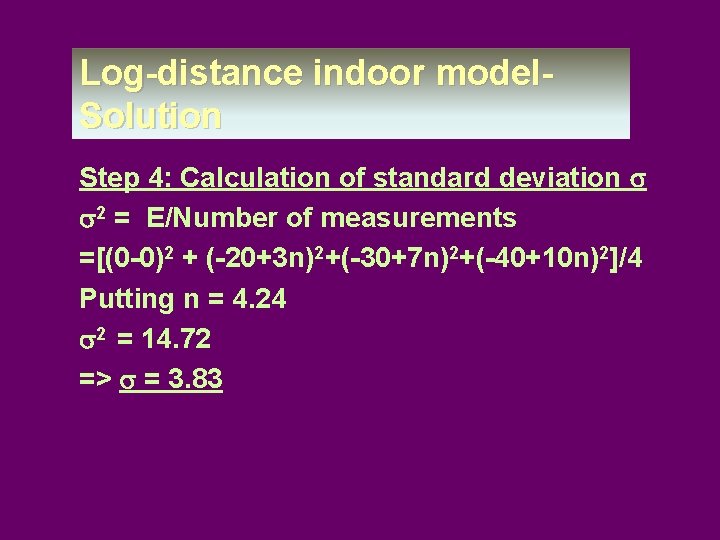
Log-distance indoor model- Solution Step 4: Calculation of standard deviation s s 2 = E/Number of measurements =[(0 -0)2 + (-20+3 n)2+(-30+7 n)2+(-40+10 n)2]/4 Putting n = 4. 24 s 2 = 14. 72 => s = 3. 83

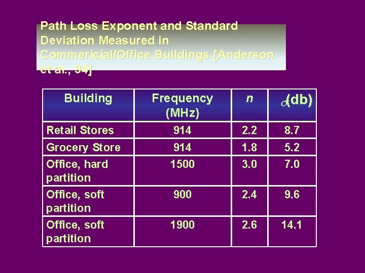
Path Loss Exponent and Standard Deviation Measured in Commericial/Office Buildings [Anderson et al. , 94] Building Frequency (MHz) n Retail Stores Grocery Store 914 2. 2 1. 8 8. 7 5. 2 Office, hard partition Office, soft partition 1500 3. 0 7. 0 900 2. 4 9. 6 1900 2. 6 14. 1 s(db)

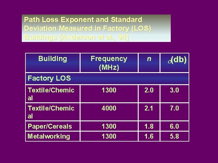
Path Loss Exponent and Standard Deviation Measured in Factory (LOS) Buildings [Anderson et al. , 94] Building Frequency (MHz) n 1300 2. 0 3. 0 4000 2. 1 7. 0 1300 1. 8 1. 6 6. 0 5. 8 s(db) Factory LOS Textile/Chemic al Paper/Cereals Metalworking

Path Loss Exponent and Standard Deviation Measured in Home/Factory (OBS)Buildings [Anderson et al. 94] Building Frequency (MHz) n Indoor to Street Factory OBS 900 3. 0 7. 0 Textile/Chemic al Metalworking 4000 2. 1 9. 7 1300 3. 3 6. 8 s(db) Suburban Home

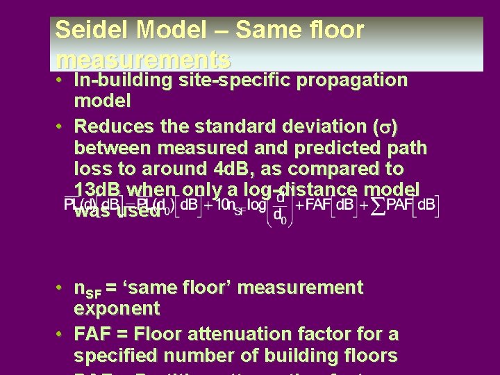
Seidel Model – Same floor measurements • In-building site-specific propagation model • Reduces the standard deviation (s) between measured and predicted path loss to around 4 d. B, as compared to 13 d. B when only a log-distance model was used • n. SF = ‘same floor’ measurement exponent • FAF = Floor attenuation factor for a specified number of building floors

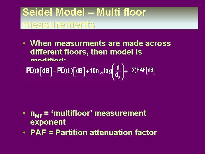
Seidel Model – Multi floor measurements • When measurments are made across different floors, then model is modified: • n. MF = ‘multifloor’ measurement exponent • PAF = Partition attenuation factor

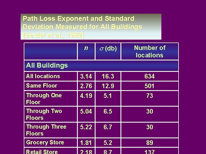
Path Loss Exponent and Standard Deviation Measured for All Buildings [Seidel et al. , 1992] n s (db) Number of locations 3. 14 2. 76 16. 3 12. 9 634 501 Through One Floor 4. 19 5. 1 73 Through Two Floors 5. 04 6. 5 30 Through Three Floors 5. 22 6. 7 30 Grocery Store 1. 81 5. 2 89 All Buildings All locations Same Floor

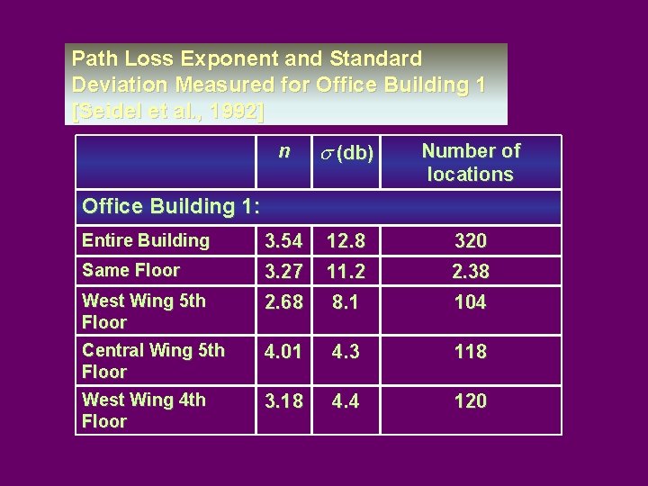
Path Loss Exponent and Standard Deviation Measured for Office Building 1 [Seidel et al. , 1992] n s (db) Number of locations 3. 54 3. 27 12. 8 11. 2 320 2. 38 West Wing 5 th Floor 2. 68 8. 1 104 Central Wing 5 th Floor 4. 01 4. 3 118 West Wing 4 th Floor 3. 18 4. 4 120 Office Building 1: Entire Building Same Floor

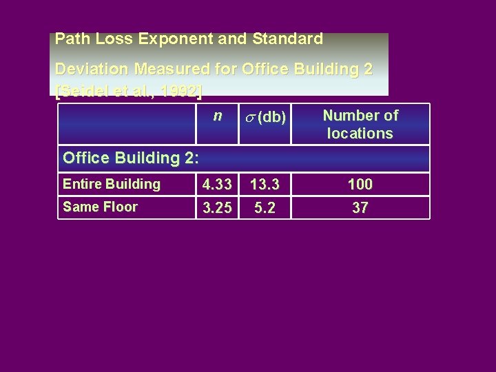
Path Loss Exponent and Standard Deviation Measured for Office Building 2 [Seidel et al. , 1992] n s (db) Number of locations 4. 33 3. 25 13. 3 5. 2 100 37 Office Building 2: Entire Building Same Floor

Free-space plus linear Path Attenuation Model [Devasirvathan et al, 90] - Attenuation constant for channel (d. B/n) FAF- Floor attentuation factor PAF- Partition attentuation factor

Free Space Plus Linear Path Attenuation Model parameters [Devasirvathan et al, 90] Location Building 1: 4 story Building 2: 2 story Frequency a —Attenuation 850 MHz (d. B/m) 0. 62 1. 7 GHz 4. 0 GHz 0. 57 0. 47 850 MHz 0. 48 1. 7 GHz 4. 0 GHz 0. 35 0. 23