Practical Loop Tuning How to Tune a PID

Practical Loop Tuning – How to Tune a PID Loop! 2015 ATMAE Conference (EECT Track) Pittsburgh, Pennsylvania John R. Wright, Jr. , Ph. D. , CSTM Department of Applied Engineering, Safety, and Technology Millersville University

Need n “PID controllers have been at the heart of control engineering practice for seven decades. In process control, more than 95% of the control loops are of the Proportional-Integral-Derivative (PID) type” (Raut & Vaishnav, 2014). n With more than 200 different algorithms available on how to tune a control loop, tuning a loop can be daunting, if not confusing. Many controls professionals even consider the process of tuning a loop a black art due to the complexity involved. n Applied engineers need to understand the basics of PID closed loop control and how to practically tune a loop in the field as they are often faced with this challenge as process, manufacturing, and controls engineers.

PID Elements n. P – Proportional n. I – Integral n. D – Derivative

Proportional Control n A corrective force that is proportional to the amount of error. CO = KPE + Bias CO = Controller Output due to proportional control KP = proportional constant for the system called gain E = error § Where E = Set Point (SP) – Process Variable (PV) (Reverse Acting)* § Where E = Process Variable (PV) – Set Point (SP) (Direct Acting)* *Some Controllers do not allow for negative gain values Bias = used to remove the steady state error at a particular set point § If we have zero error, our proportional term will contribute zero to the controller output. Without error, a proportional controller does nothing! Bias is used to ensure this is true.

Proportional Control n Acts in the now - what is my error now? n Is used for fast responding processes that do not require offset free operation (some specific level, pressure, etc. ) n Proportional Control Example: – Control Output moves actuator to reduce error. As the error becomes less, so does the output until the set point is reached.

Proportional Control n Steady-State-Error – Main problem of proportional control – when error is close to zero, the force becomes small and is not enough to overcome friction - stops before set point. § Dead band or dead zone: area on both sides of set point – Friction, backlash, flexing parts, poor controller design – Bias sometimes used to prevent this or one could increase the gain, but this may cause oscillations

Proportional-Integral Control n n Creates a restoring force that is proportional to the sum of all past errors multiplied by time. Whereas proportional control works in the present (what is my error now), integral action works in the past for integral control action sums the error over all past time and multiplies this summed error value times the tuning parameter. Integral can be used alone (Very Sluggish), but is normally used with proportional control for better responsiveness. PI control is used for fast responding processes that require offset free operation.

Proportional-Integral Control CO = KP [E + KI (E t)] CO = Controller Output due to proportionalintegral control KP = proportional gain constant KI = integral gain constant (E t) = sum of all past errors (multiplied by the time they existed)

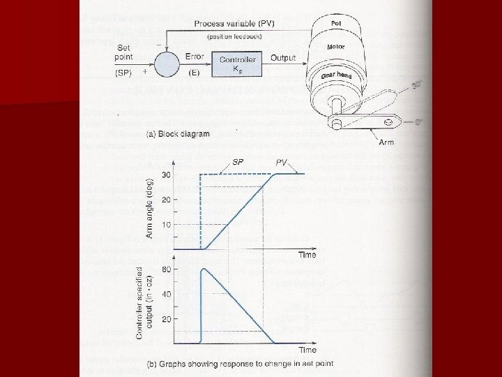
Integral Control n Integral control is used to reduce steady-state error to zero. – For a constant value of error, the value of (E t) will increase with time causing the restoring force to get larger and larger. – Eventually, the restoring force will get large enough to overcome friction and move the controlled variable in a direction to eliminate the error. § Example (next slide) Integral control slowly increases torque, and after 5 seconds, moves the last 2° to eliminate the error.

Integral Example n Integral control increases by 2 in. *oz every time period.

“Integral response can easily be observed on industrial robots. When a weight is placed on the arm, it will visibly sag and then restore itself to the original position. ”

Problems with Integral Control Reduced stability n Oscillations n Slow: It takes time for error*time to accumulate. n

Proportional-Integral-Derivative Control n Applies the brakes, slowing the controlled variable just before it reaches its destination. n If proportional works in the present, and integral works in the past, derivative works by trying to anticipate the future. n Derivative action is never used by itself. It is always used with P or PI. n Derivative will allow you to used higher controller gains or can further smooth out integral instability.

Proportional-Integral-Derivative Control CO = KP [E + KI (E t) + KD ( PV / t)] CO = Controller Output due to proportional-integralderivative control KP = proportional gain constant KI = integral gain constant KD = derivative gain constant (E t) = sum of all past errors (multiplied by the time they existed) ( PV/ t) = error rate of change (slope of error curve) § Remember PV = Process Variable (sensor reading)

Derivative Control n n Derivative control is a solution to the overshoot problem. Slows down the controlled variable to minimize overshoot. Derivative control is Proportional to error slope. Helps systems respond quicker to changes in the load.

Derivative Control n Improves system in 2 ways: – Extra force to start. – Provides brakes to slow down when close to set point. Too much derivative control can cause slow system response. n Can can valve chatter! n Never used by itself n

Know Your Process (Self-regulating vs. Integrating) n Self-regulating – Cruise Control – Flow Control – Continuous Temp Control – Steam Pressure with Variable Flow Output http: //www. controlguru. com/postpics/integratingbehavior. jpg NOTE: In Open Loop – step the output of the controller and observe

Know Your Process (Self-regulating vs. Integrating) n Integrating – Batch Temp Control Systems – Level Control Systems – Steam Pressure with Fixed Flow Output http: //www. controlguru. com/postpics/integratingbehavior. jpg NOTE: In Open Loop – step the output of the controller and observe (does not return like self-regulating or lags significantly)

Know Your Controller http: //www. pidtuning. net/img/alg-types. png

Know Your Controller (Series or Classical) http: //www. pidtuning. net/img/alg-types. png This is what most engineers study for PID Control Theory – was the first type of PID control. It is a nightmare to tune by trial and error as the terms affect each other. A change in P affects the I and D and so on…

Know Your Controller (Parallel) http: //www. pidtuning. net/img/alg-types. png All three are independent – results are added at the end

Know Your Controller (Ideal or ISA) http: //www. pidtuning. net/img/alg-types. png Not too bad to tune – most controllers today use this method of control including Allen Bradley PLCs We will focus on this method for the presentation!

Relationship Between K & T n K = “gain” & T = “time” § KP=K § KI=K/Ti § KD=K*Td n While we used K to describe the terms in the tuning equations, controllers may ask for either the T or K for integral and derivative terms n We will be solving for T, but one may convert this should it be required

Allen Bradley Practical Process Control: Fundamentals of Instrumentation and Process Control Station

Tuning Methods & Response n Zeigler-Nichols ¼ Wave Decay http: //www. jashaw. com/pid/tutorial/pid 6. html n Pessen Little or No Overshoot http: //www. valin. com/sites/default/files/valve-flow 2 -fig 4_1. jpg

Zeigler-Nichols Approach n John G. Zeigler and Nathaniel B. Nichols are the fathers of scientific tuning methods – In 1942, they published two loop tuning techniques that addressed the question of how an engineer can determine the values of Kp, Ti, and Td n ¼ Wave decay concept § Criticism is that it will not give robust controller performance and the process borders on instability

ZN Methods n 1) Z-N Continuous Cycling Method – This is a trial and error method conducted while a control loop is in automatic mode (closed loop systems) n 2) Z-N Step Method – Uses a reaction curve to perform calculations – Used for stable open loop systems (manual mode)

Z-N Continuous Steps n Step 1 § With the loop in automatic mode, enter a new set point a small amount above or below the set point at which you want to tune. Allow the loop to stabilize. n Step 2 § Place the loop in manual mode, the loop must continue to be stable. n Step 3 § Turn off integral and derivative action (set them to zero), and set proportional to a small value. n Step 4 § Place the controller in automatic mode.

Z-N Continuous Steps n Step 5 n Step 6 n Step 7 n Step 8 § Change the set point (SP) to your operating set point, an offset should occur in the process variable (PV). § Increase the gain until the loop starts oscillating. http: //www. jashaw. com/pid/tutorial/pid 6. html § Record the gain as your ultimate gain (Ku). § Record the resulting period as the ultimate period (Pu).

Z-N Continuous Steps n Step 9 § Calculate Kp, Ti, and Td using the following table: Kp Ti Td P 0. 50 KU — — PI 0. 45 KU Pu /1. 2 — PID 0. 60 KU Pu /2 Pu /8

Z-N Continuous Method n Even though this method is frequently used, it has the following disadvantages: § It can be time consuming if several trials are required and the process dynamics are slow. § Introducing oscillations into a process is in many cases not desirable. § Will not work for an integrating process. – Some processes where the streams are comprised of gases, liquids, powders, slurries and melts do not naturally settle out at a steady state operating level. Process control practitioners refer to these as non-self regulating, or more commonly, as integrating processes. (http: //www. controlguru. com/wp/p 79. html) § Will not work for dead time dominant processes. – Dead time is the delay from when a controller output (CO) signal is issued until when the measured process variable (PV) first begins to respond. The presence of dead time, Өp, is never a good thing in a control loop. (http: //www. controlguru. com/wp/p 79. html) § Requires proper manipulation of the bias value by the controller or the person doing the tuning.

Z-N Step Method n Step 1 § Create a disturbance (Δ CV) -- Step Function the system input n Step 2 § Record this on a Reaction Curve (Graph) n Step 3 § Draw a line tangent to the rising part of the response curve. This line defines the lag time (L) and rise time (T) values. – Lag time is the time delay between the controller output and the CV response

Z-N Step Method n Step 4 § Calculate the slope of the curve (Refer to example on next few slides) n Step 5 § Calculate the PID constants (Refer to example on next few slides)

L =. 2 s (lag time) T =. 9 s (rise time) PV = 7% (change in process variable from sensor) CV = 10% (step change of controlled variable from controller)

Z-N Step Method (STEP 5) N = slope of response curve L =. 2 s (lag time) T =. 9 s (rise time) PV = 7% (change in process variable from sensor) CV = 10% (step change of controlled variable from controller) N = ( PV)/T = 7%/. 9 s = 7. 8%/s Kp = (1. 2 CV)/NL = (1. 2*10%)/(7. 8%/s*. 2 s) = 7. 7 Ti = 1/2 L = 1/(2*. 2 s) = 2. 5/s Td =. 5 L =. 5*2 s =. 1 s

Pessen Tuning Approach Pessen uses the same approach as Z-N continuous cycling method, determining the ultimate process gain and ultimate process period through trial and error. n Pessen modifies the Z-N calculations to achieve either no overshoot or some overshoot. n No Overshoot Some Overshoot Kp = 0. 2 Ku Kp = 0. 33 Ku Ti = Pu / 3 Ti = Pu / 2 Td = Pu / 2 Td = Pu / 3

Tuning a Cascade Loop n Loop within a Loop n No more difficult than a regular loop. n Tune from inside out – Master Loop (outside loop) – Slave Loop (inner loop) – The master loop is the one that receives the input to the process – The output of the master loop is the input (Set Point) for the slave loop – The Slave Loop sends its output to the final control element – Slave Loop first (usually P only as it must be quick)

For Integrating Processes “One of the biggest challenges for practitioners is recognizing that a particular process shows integrating behavior prior to starting a controller design and tuning project. This, like most things, comes with training, experience and practice. Once in automatic, closed loop behavior of an integrating process can be unintuitive and even confounding. Trial and error tuning can lead us in circles as we try to understand what is causing the problem” (Rice & Cooper, 2007). http: //www. controlguru. com/wp/p 79. html n Consider using a Proportional only type control

Any Questions? n Presentation available on my website: www. millersville. edu/~jwright

References Dunning, G. (2006). Introduction to Programmable Logic Controllers 3 rd ed. Delmar Kilian, C. (2006). Modern Control Technology 3 rd ed. Delmar n. a. (2005). Practical Process Control: Fundamentals of Instrumentation and Process Control Station Raut, K. H. & Vaishnav, S. R. (2014). Performance Analysis of PID Tuning Techniques based on Time Response Specification. International Journal o. F Innovative Research IN Electrical, Electronics, Instrumentation and Control Engineering Vol. 2(1) Rhoads, H. (2005). Introduction to Process Control, The Hershey Company Rice, B. & Cooper, D. (2015). Recognizing Integrating (Non-Self Regulating) Process Behavior. Controlguru. com