Power law processes and nonextensive statistical mechanics some

Power law processes and nonextensive statistical mechanics: some possible hydrological interpretations. Chris Keylock

Talk Outline (1)Classical and nonextensive statistical mechanics (2)Power-law processes in drainage networks (3)Applying nonextensive statistical mechanics to historical flood data – the case of the Po river (4)Hurst exponents and hydrologic time-series (5)TOPMODEL and spatial distributiveness

Classical statistical mechanics due to Boltzmann and Gibbs is one of the cornerstones of modern physics. Boltzmann (1867) linked macroscopic properties of a phenomenon (temperature, entropy) to microscopic probabilities to lay the foundations for the contemporary subdiscipline of statistical mechanics. Subsequently, this has become an extremely powerful tool for a variety of problems.

Determining the range of validity of this thermodynamics is not a simple problem. Krylov (1944) suggested that the property of mixing was at the heart of the this question. Quick (exponential) mixing leads to a short relaxation time. It results in strongly chaotic behaviour (positive Lyapunov exponent). However, one can also have slower (power-law) mixing processes that are weakly chaotic. The difference emerges because of short (long) ranged interactions and smooth (complex i. e. fractal/multifractal) boundary conditions. Krylov N. 1944. Nature 153, 709.

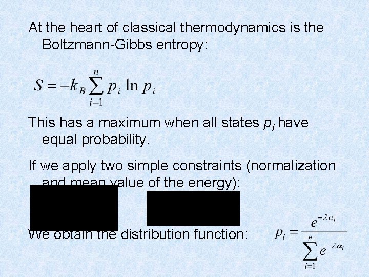
At the heart of classical thermodynamics is the Boltzmann-Gibbs entropy: This has a maximum when all states pi have equal probability. If we apply two simple constraints (normalization and mean value of the energy): We obtain the distribution function:

However, in river systems there is a great deal of evidence for power-law and multifractal behaviour rather than exponential. There is a whole book that describes a variety of aspects of this (Rodriguez-Iturbe and Rinaldo, 1997). In particular, perhaps the network width function is important in this context. It gives the number of links in the basin as a function of distance from the outlet and has been shown to be multifractal. The width function has been used for flood prediction and for defining the geomorphic instantaneous unit hydrograph. Rodriguez-Iturbe I. , Rinaldo I. 1997. Fractal River Basins: Chance and selforganization. Cambridge University Press.

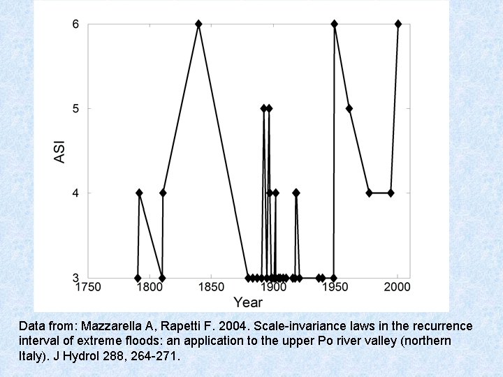
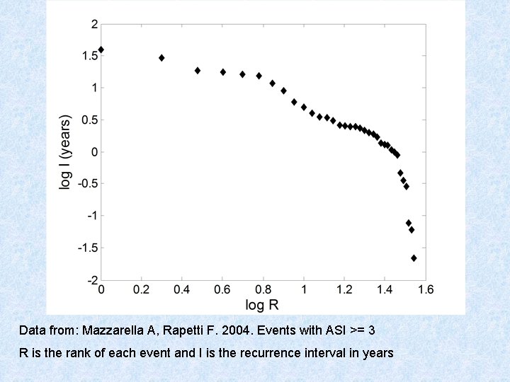
Data from: Mazzarella A, Rapetti F. 2004. Scale-invariance laws in the recurrence interval of extreme floods: an application to the upper Po river valley (northern Italy). J Hydrol 288, 264 -271.

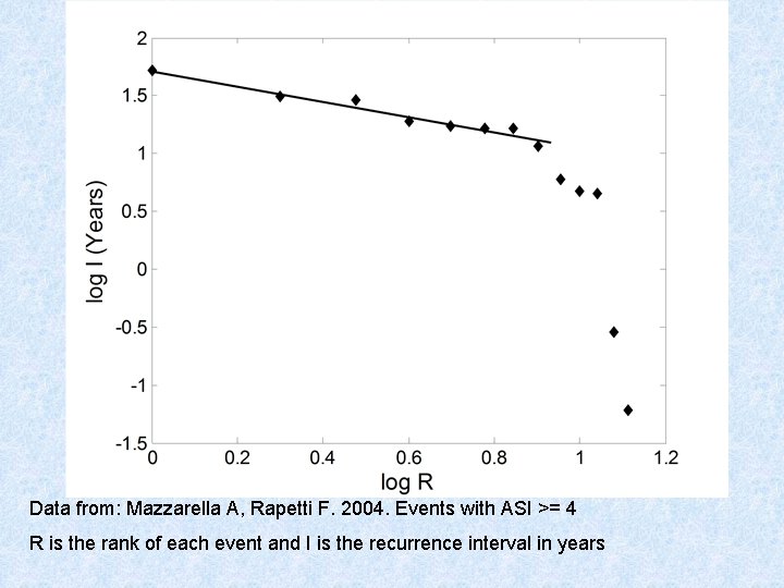
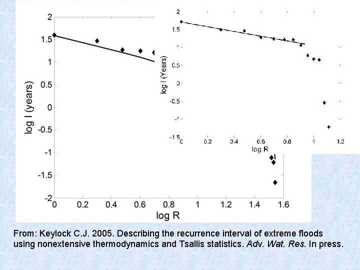
Data from: Mazzarella A, Rapetti F. 2004. Events with ASI >= 4 R is the rank of each event and I is the recurrence interval in years

Data from: Mazzarella A, Rapetti F. 2004. Events with ASI >= 3 R is the rank of each event and I is the recurrence interval in years

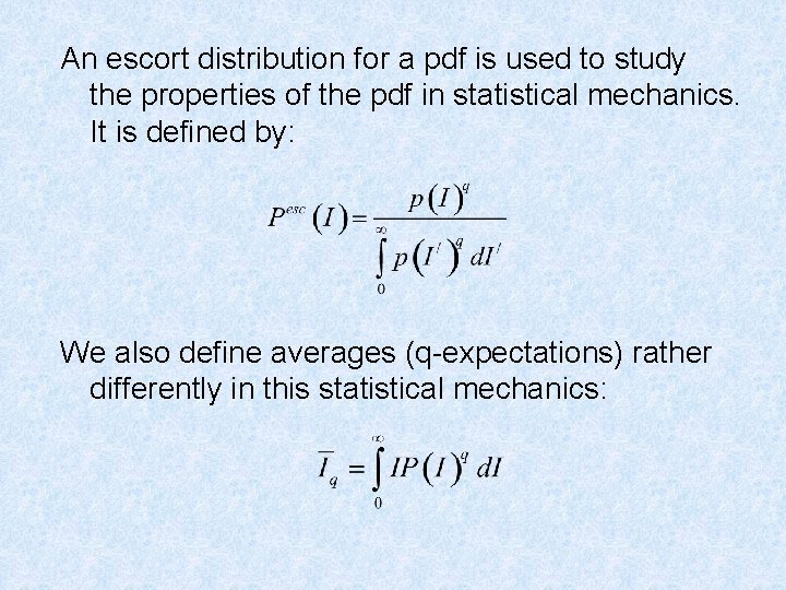
An escort distribution for a pdf is used to study the properties of the pdf in statistical mechanics. It is defined by: We also define averages (q-expectations) rather differently in this statistical mechanics:

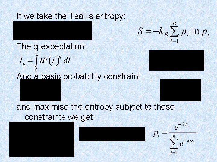
If we take the Tsallis entropy: The q-expectation: And a basic probability constraint: and maximise the entropy subject to these constraints we get:

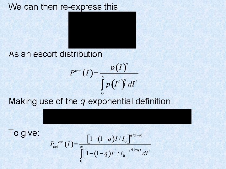
We can then re-express this As an escort distribution Making use of the q-exponential definition: To give:

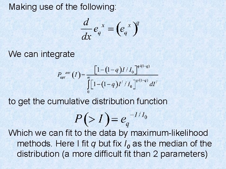
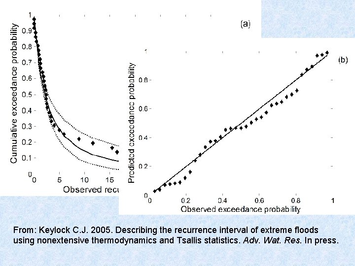
Making use of the following: We can integrate to get the cumulative distribution function Which we can fit to the data by maximum-likelihood methods. Here I fit q but fix I 0 as the median of the distribution (a more difficult fit than 2 parameters)

From: Keylock C. J. 2005. Describing the recurrence interval of extreme floods using nonextensive thermodynamics and Tsallis statistics. Adv. Wat. Res. In press.

From: Keylock C. J. 2005. Describing the recurrence interval of extreme floods using nonextensive thermodynamics and Tsallis statistics. Adv. Wat. Res. In press.

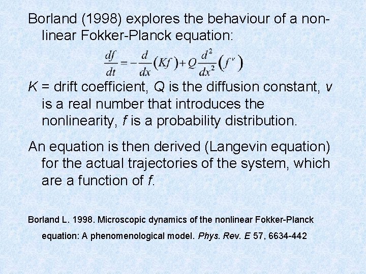
There is a direct connection between this entropic form and correlated anomalous diffusion that is described by nonlinear Fokker-Planck equations (Borland, 1998). Consequently, data that can be described by the q-exponential distribution may be generated by the relevant underpinning differential equation. Borland L. Microscopic dynamics of the nonlinear Fokker-Planck equation: A phenomenological model. Phys Rev E 1998; 57: 6634 -6642.

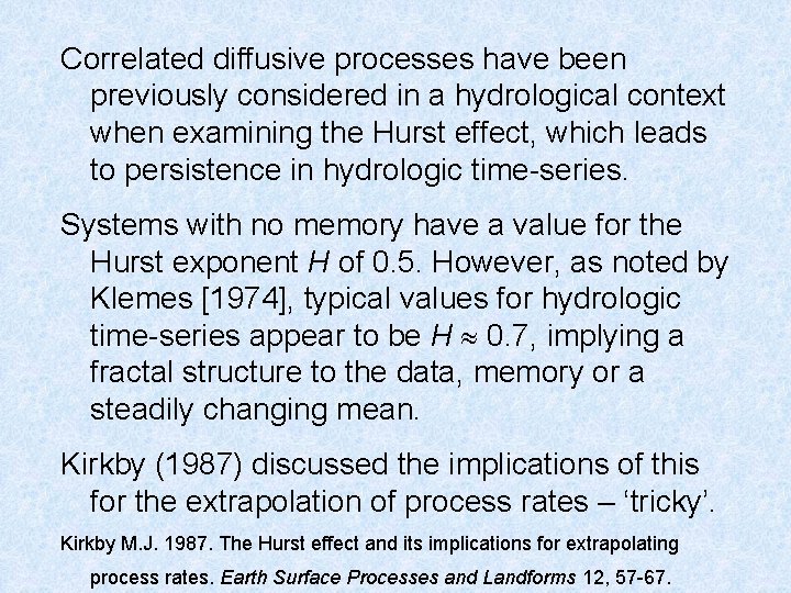
Correlated diffusive processes have been previously considered in a hydrological context when examining the Hurst effect, which leads to persistence in hydrologic time-series. Systems with no memory have a value for the Hurst exponent H of 0. 5. However, as noted by Klemes [1974], typical values for hydrologic time-series appear to be H 0. 7, implying a fractal structure to the data, memory or a steadily changing mean. Kirkby (1987) discussed the implications of this for the extrapolation of process rates – ‘tricky’. Kirkby M. J. 1987. The Hurst effect and its implications for extrapolating process rates. Earth Surface Processes and Landforms 12, 57 -67.

Borland (1998) explores the behaviour of a nonlinear Fokker-Planck equation: K = drift coefficient, Q is the diffusion constant, ν is a real number that introduces the nonlinearity, f is a probability distribution. An equation is then derived (Langevin equation) for the actual trajectories of the system, which are a function of f. Borland L. 1998. Microscopic dynamics of the nonlinear Fokker-Planck equation: A phenomenological model. Phys. Rev. E 57, 6634 -442

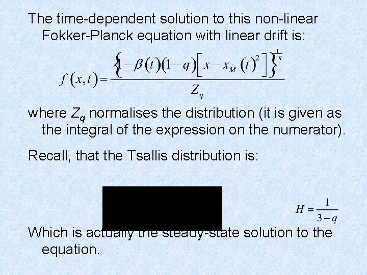
The time-dependent solution to this non-linear Fokker-Planck equation with linear drift is: where Zq normalises the distribution (it is given as the integral of the expression on the numerator). Recall, that the Tsallis distribution is: Which is actually the steady-state solution to the equation.

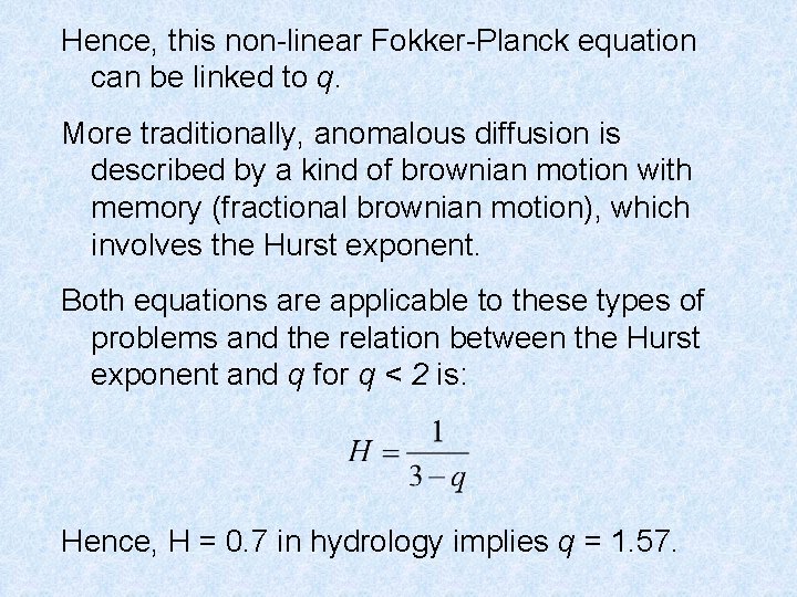
Hence, this non-linear Fokker-Planck equation can be linked to q. More traditionally, anomalous diffusion is described by a kind of brownian motion with memory (fractional brownian motion), which involves the Hurst exponent. Both equations are applicable to these types of problems and the relation between the Hurst exponent and q for q < 2 is: Hence, H = 0. 7 in hydrology implies q = 1. 57.

An important part of the classic version of TOPMODEL is the topographic index given by Ln (a / tan β) where a is the upslope area per unit contour length and tan β is the surface slope. (e. g. Lane et al. , 2004 for a modification). Recently, Ambroise et al. (1996) and others have proposed generalisations of this to deal with different catchment characteristics (e. g. parabolic and linear transmissivity profiles). Ambroise B. , Beven K. , Freer J. 1996. Toward a generalization of the TOPMODEL concepts: Topographic indices of hydrological similarity, Water Resources Research 32, 2135 -2145. Lane SN, Brookes CJ, Kirkby MJ, Holden J. 2004. A network-index based version of TOPMODEL for use with high-resolution digital topographic data. Hydrological Processes 18, 191 -201.

Kirkby (1997) argues that a move away from the exponential treatment of the relation between discharge and soil moisture may mean that spatially explicit solutions to the equations for TOPMODEL become necessary. Based on the framework presented here, it may be possible to construct the same argument from a different starting point. Unless one uses the logarithmic form of the index, you are implying a slow mixing of an appropriate intensive quantity of the hydrological system. The associated complexity introduced by this slow mixing implies a spatially explicit solution. Kirkby M. J. 1997. TOPMODEL: A personal view. Hydrological Processes 11, 1087 -97.