POTENTIAL METHODS 2020 2021 Part 5 Magnetic field

POTENTIAL METHODS 2020 -2021 Part 5 Magnetic field Carla Braitenberg Trieste University, DMG Home page: http: //www 2. units. it/~braitenberg/ e-mail: berg@units. it 1

The earth’s magnetic field and potential § § § Topics Definition of magnetic potential of dipole source Spherical harmonic expansion of the Earth inner magnetic potential field Definition of Earth Magnetic Reference Field Definition of Magnetic anomaly Induced and remanent magnetization § As further reference recommend the textbook Hinze et al. 2013. 2

Reference textbooks n Hinze, von Frese, Saad, (2013), Gravity and Magnetic Exploration, Cambridge University Press For students with mathematical foundations who are interested to explore theory of potential fields: n Blakely, R. (1996) Potential Theory in Gravity and Magnetic Applications, Cambridge University Press, New York. n 3

Magnetic potential of dipole source n Potential of dipole is the fundamental equation for modeling and inversion. Dipole is the elementary source unit. U(x, y, z) 4

Magnetic field: derivative of magnetic potential n The magnetic field, measured in A/m is obtained from the gradient of the potential. n A dipole placed in a magnetic field H senses a torque τ. The torque is proportional to the magnetic field strength and to the magnetic dipole. The torque depends also on the surrounding material, which can enhance the existing magnetic field. Therefore the magnetic induction vector B is defined, which is measured in units of Tesla (or nano Tesla, n. T): Here k is termed the magnetic susceptibility, which is a adimensional property of the material. n We also need a physical constant to relate the field strength to the torque, which is the permeability of free space: n n n 5 The torque (measured in Nm) is given by: Fine lezione 22 dic 2020

Magnetization n 6 The term that adds to the magnetic field is called the magnetization. It has the same units as the magnetic field (A/m) and is a vector quantity. It can be interpreted as the number of dipoles per unit volume, because it is due to an alignment of existing material dipoles.

First approximation of Earth magnetic field As a first approximation the Earth’s magnetic field is described as a dipole field. This is though a crude approximation and insufficient for geophysical prospecting purposes. Rather a higher order reference field is used in terms of spherical harmonic expansion as the reference field. n It is the International Geomagnetic Reference Field. n It is produced as a Spherical harmonic expansion of the reference field n Anomaly: observed field‐reference field. n Reference field: should eliminate field unrelated to crustal magnetic sources. n Spherical harmonic expansion of global field. As field varies in time, it is defined every 5 years, together with the time derivative. Intermediate fields are calculated by linear interpolation. n Frese et al. (2013) 7 Prof. Carla Braitenberg

IGRF 13° generation just published in December 2019, valid for 1900‐ 2025 n Published Reference: International Geomagnetic Reference Field: the 12 th generation, Erwan Thébault, Christopher C Finlay, Ciarán D Beggan, et al. Earth, Planets and Space 2015, 67: 79 (27 May 2015) n Link: https: //www. ngdc. noaa. gov/IAGA/vmod/igrf. html n 8

Spherical harmonic development inner magnetic field- as IGRF n The magnetic potential field: Gauss coefficients in n. T Associated Legendre Polynome r= radial distance from Earth center, a= 6371. 2 km (equatorial radius) N= 10 up to epoch 1995, N=13 for epochs 2000, 2005, …, 2020 n 9 The magnetic induction vector. Notice the similarity to the formalism we have discussed for the Earth gravity field:

Sign Conventions for the three components of the magnetic field vector X=Horizontal North component, positive northwards n Y= Horizontal East Component, positive eastwards n Z= Vertical component, positive downwards n 10

Magnetic field Inclination (IGRF 12) Thébault et al. 2015

Total Magnetic field (IGRF 12) Thébault et al. 2015

Magnetic field Declination (IGRF 12) Thébault et al. 2015

Magnetic field Inclination change rate (IGRF 12) Thébault et al. 2015

Total Magnetic field change rate (IGRF 12) Thébault et al. 2015

Magnetic field Declination change rate (IGRF 12) Thébault et al. 2015

Magnetic field change in north and south pole (IGRF 12) Thébault et al. 2015

Define Anomaly n n n 18 Anomaly: observed field minus reference field. Reference field: should eliminate field unrelated to crustal magnetic sources. IGRF: used as non‐crustal magnetic field The spectral analysis shows a knee of the spectral amplitude curve at about N=13 to N=15 according to different authors. next graph of Maus(2008) refers to the N=15 knee. Depends on the way of averaging the spectrum on the sphere.

Define Total Field Anomaly § Field observations involve total field. § Anomalous field is in the order of 102 n. T , normal field is in the order of 2 -6 104 n. T, so observed and reference fields near to parallel. Therefore define anomaly as difference between magnitudes of both vectors.

Spectral analysis: internal and crustal magnetic field Geomagnetic power spectrum: global model NGDC-720 compared to subsets of World Magnetic Anomaly Map (NGDC). Maus, 2008. In next page the degree power Sn is defined.

Define power spectrum of magnetic field The power spectrum Sn at degree n of the field B is defined as the scalar product Bn Bn averaged over the surface of the sphere with radius a: Use the expression of Bn and the orthogonality of the spherical harmonic functions The power spectrum for a particular degree n can be shown to become: Robert Van Der Hilst. 12. 201 Essentials of Geophysics, Fall 2004. (Massachusetts Institute of Technology: MIT Open. Course. Ware), http: //ocw. mit. edu (Accessed 2 Dec, 2015). License: Creative Commons BY-NC-SA

Crustal field

Crustal field due to magnetisation of the rocks

Remanent magnetization § Rock can have remanent magnetization acquired during a § § § heating event. Remanent magnetization is oriented along field of time of heating Orientation: regional property if heating was regional Classical remanent magnetization: ocean bottom, with remanent magnetization aligned in stripes.

Induced and remanent magnetization § In a practical study, the total magnetization of the rock should be considered as the vector sum of its induced and remanent magnetization. Königsberger ratio: ratio of amount of remanent and induced magnetization. Modeling: if remnancy unknown, start with modeling only induced magnetization. Add correction for remnancy at the end. § Mafic rocks (e. g. basalt) are more magnetic than silicic rocks. Extrusive rocks have a higher remanent magnetization and lower susceptibility than intrusive rocks with the same chemical composition. Sedimentary and metamorphic rocks often have low remanent magnetization and susceptibilities.

Susceptibility changes for varying percentages of minerals. Notice that either volume percent or weight percent is used in the graph. 26

Total field anomaly of the magnetized sphere § The total field anomaly is equal to the projection of the anomalous magnetic field along the direction of the inducing field. In formula, with the inducing field having direction given by vector the magnetic induction vector at the position vector , with being centered on the sphere, is the follwowing: Magnetic field induction vector: Total magnetic field anomaly:

Vertical inducing field as at North-pole (section in the x-z plane)

Vertical inducing field as at North-pole (profiles) Inclination=90° X-axis from South to North

Inducing field at mid-latitudes Northern hemisphere (Inclination=60°)

Inducing field at mid-latitudes Northern hemisphere (profiles) (Inclination=60°) X-axis from South to North

Inducing field at mid-latitudes Northern hemisphere (Inclination=0°)

Inducing field at magnetic equator (profiles) (Inclination=0°) X-axis from South to North

Field study Italy-Lazium anomalies Volcanic edifices: Vulsini, Vico, Sabatini, Albani Age: Miocene‐Quaternary (Latium: began: 0. 4‐ 0. 6 Ma, ended 0. 1 Ma; Albani: began 0. 02 Ma). Age is recent, so remanent field is assumed to be aligned to today‘s field. Caratori Tontini et al. , 2006, JGR

Inversion result The magnetic susceptibility is shown from the surface down to a depth of 13500 m. The magnetic susceptibility has benn optimized to fit the magnetic field observations. Caratori Tontini et al. , 2006, JGR

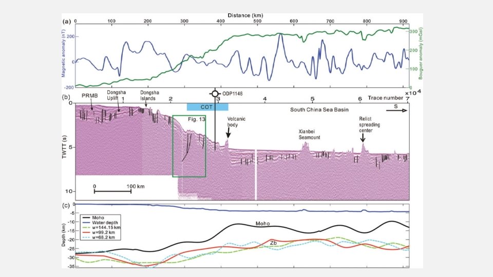
Tectonic outline- field study South China Sea Li et al. , 2010. Depths to the magnetic layer bottom in the South China Sea area and their tectonic implications, Geophys. J. Int. , doi: 10. 1111/j. 1365‐ 246 X. 2010. 04702. x

Magnetic field Map of total field magnetic anomalies in the SCS area.

Bottom of magnetic sources through spectral analysis. 100 km square windows

Moho depth from simple gravity inversion

References Caratori Tontini F. , L. Cocchi, C. Carmisciano (2006) Depth‐to‐the‐bottom optimization for magnetic data inversion: Magnetic structure of the Latium volcanic region, Italy, https: //doi. org/10. 1029/2005 JB 004109 n Li et al. , 2010. Depths to the magnetic layer bottom in the South China Sea area and their tectonic implications, Geophys. J. Int. , doi: 10. 1111/j. 1365‐ 246 X. 2010. 04702. x n Thébault et al. Earth, Planets and Space (2015) 67: 79, DOI 10. 1186/s 40623‐ 015‐ 0228‐ 9 n