Pose Estimation OHAD MOSAFI Motivation Detecting people in

Pose Estimation OHAD MOSAFI

Motivation §Detecting people in images is a key problem for video indexing, browsing and retrieval. § the main difficulties are the large appearance variations caused by action, clothing, illumination, viewpoint and scale.

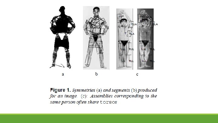
Finding people by sampling §People can be quite accurately modeled as assemblies of cylinders and these assemblies are constrained by the kinematics of human joints. §People are presented as collections of nine body segments one for the torso and two for each limb.

Finding people by sampling §Symmetries- pairs of edge elements that are approximately symmetric about some symmetry axis and whose tangents are approximately parallel to that axis. §Segments- extended group of symmetries which approximately share the same axis (expectation- maximization algorithm that assumes a fixed number of segments). §Using learned likelihood model to form assemblies by sampling. §Finally the set of assemblies is replaced with a smaller set of representatives, which are used to count people in the image.

Thumbtack

Maximum Likelihood

Maximum Likelihood

Maximum Likelihood

Log-likelihood

Log-likelihood

Log-likelihood <- -> Likelihood Reconsider thumbtack: 8 up, 2 down.

Log-likelihood <- -> Likelihood

Finding Segments Using EM A symmetry fits a segment best when the midpoint of the symmetry lies on the segment’s symmetry axis, the endpoints lie half a segment width away from the axis, and the symmetry is perpendicular to the axis This yields the conditional likelihood for a symmetry given a segment as a four-dimensional Gaussian, and an EM algorithm can now fit a fixed number of segments to the symmetries.

Mixture of Gaussians

Mixture of Gaussians

Expectation Maximization

Expectation Maximization

EM Derivation

EM Derivation(cont. )

Jensen’s inequality

EM Derivation(cont. )

EM for Mixture of Gaussians

EM for Mixture of Gaussians

EM for Mixture of Gaussians

Representing Likelihood for people

Marginal Likelihood

Building Assemblies Incrementally by Resampling

Building Assemblies Incrementally by Resampling (cont)

Directing the Sampler

Example

Example(cont. ) §Now let us supposed that we have fixed a torso and, possible, some limbs, and we want to add the left arm that would maximize the likelihood of the result. §First, we will find the highest-likelihood left arm for each choice of the upper arm. Since no feature involves the left arm and any other limb, we can choose the best left arm by considering all the pairs of torso(fixed) and a left arm, and choosing the one with the largest marginal likelihood.

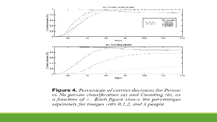
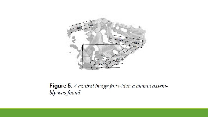
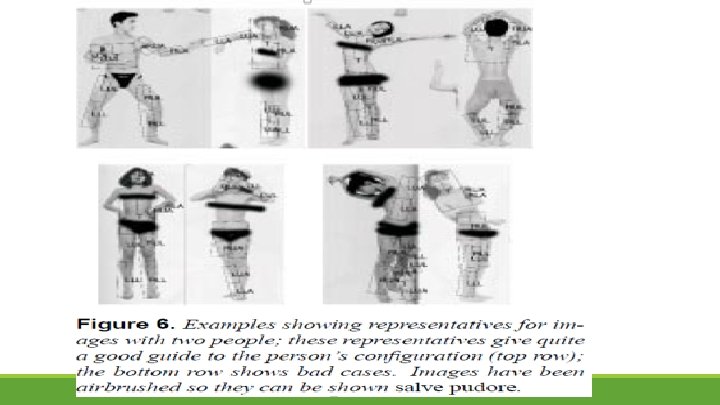
Counting people §This sampling algorithm allows to count people in images. To estimate the number of people. We begin by selecting a small set of representative assemblies in the image and then use them for counting §We break the set of all assemblies in the image into (not necessarily disjoint) blocks — sets of assemblies such that any two assemblies from the same block have overlapping torsos. Then, the representative is chosen from each block as the assembly with the highest likelihood, over all assemblies available from the block.

Results §To learn the likelihood model , they used a set of 193 training images. (standing against a uniform background, all the views were frontal and all limbs were visible, although the configurations varied). §The training set was expanded by adding the mirror image of each assembly, thus resulting in 386 configurations. §The test set included: o 145 control images with no people o 228 – 1 people, 72 - 2 people, 65 – 3 people. (COREL database)

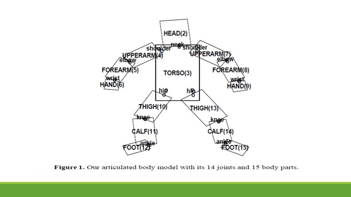
Pictorial Structure of People

Pictorial Structure of People

Detecting Body Parts The ultimate goal is to detect people and label them with detailed part locations, in applications where the person may be in any pose and partly occluded. Detecting and labelling body parts is a central problem in all component-based approaches. Clearly the image must be scanned at all relevant locations and scales, but there is also a question of how to handle different part orientations, especially for small, mobile, highly articulated parts such as arms and hands.

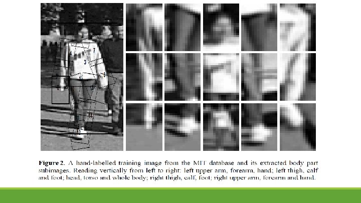
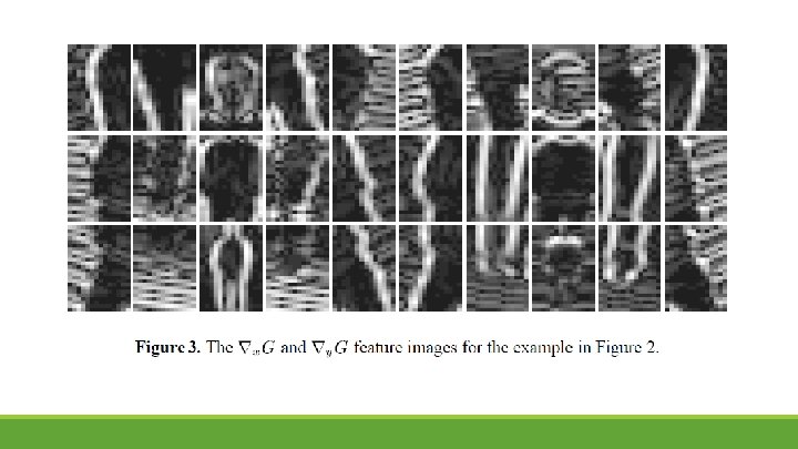
Feature Sets

Training §Using the 2016 -dimensional feature vectors for all body parts we trained two linear classifiers for each part: o Support Vector Machine o. Relevance Vector Machine. training on the smallest sets of examples that give reasonable results — in our case, about 100.

SVM- Linear Separators Binary classification can be viewed as the task of separating classes in feature space: w. Tx + b = 0 w. Tx + b > 0 w. Tx + b < 0 f(x) = sign(w. Tx + b)

Linear Separators §Which of the linear separators is optimal ?

SVM- Classification Margin Distance from example xi to the separator is Examples closest to the hyperplane are support vectors. Margin ρ of the separator is the distance between support vectors. ρ r

Maximum Margin Classification §Maximizing the margin is good according to intuition §Implies that only support vectors matter; other training examples are ignorable.

Linear SVMs Mathematically

Linear SVMs Mathematically

Linear SVMs Mathematically we can formulate the quadratic optimization problem Find w and b such that is maximized and for all (xi, yi), i=1. . n : yi(w. Txi + b) ≥ 1 Which can be reformulated as: Find w and b such that Φ(w) = ||w||2=w. Tw is minimized and for all (xi, yi), i=1. . n : yi (w. Txi + b) ≥ 1

Solving the Optimization Problem Find w and b such that Φ(w) =w. Tw is minimized and for all (xi, yi), i=1. . n : yi (w. Txi + b) ≥ 1 Need to optimize a quadratic function subject to linear constraints. Quadratic optimization problems are a well-known class of mathematical programming problems for which several (non -trivial) algorithms exist.

Solving the Optimization Problem §The solution involves constructing a dual problem where a Lagrange multiplier αi is associated with every inequality constraint in the primal (original) problem: Find α 1…αn such that Q(α) =Σαi - ½ΣΣαiαjyiyjxi. Txj is maximized and (1) Σαiyi = 0 (2) αi ≥ 0 for all αi

Quadratic Program

SVM-The Optimization Problem Solution Given a solution α 1…αn to the dual problem, solution to the primal is: w =Σαiyixi b = yk - Σαiyixi Txk for any αk > 0 Each non-zero αi indicates that corresponding xi is a support vector. Then the classifying function is (note that we don’t need w explicitly): f(x) = Σαiyixi. Tx + b Notice that it relies on an inner product between the test point x and the support vectors xi – we will return to this later. Also keep in mind that solving the optimization problem involved computing the inner products xi. Txj between all training points.

Not linearly separable cases

Soft Margin Classification §What if the training set is not linearly separable? §Slack variables ξi can be added to allow misclassification of difficult or noisy examples, resulting margin called soft.

Soft Margin Classification Mathematically §The old formulation: Find w and b such that Φ(w) =w. Tw is minimized and for all (xi , yi), i=1. . n : yi (w. Txi + b) ≥ 1

Soft Margin Classification Mathematically §Modified formulation incorporates slack variables: Find w and b such that Φ(w) =w. Tw + CΣξi is minimized and for all (xi , yi), i=1. . n : yi (w. Txi + b) ≥ 1 – ξi, , ξi ≥ 0 §Parameter C can be viewed as a way to control overfitting § it “trades off” the relative importance of maximizing the margin and fitting the training data.

Soft Margin Classification – Solution Dual problem is identical to separable case (would not be identical if the 2 -norm penalty for slack variables CΣξi 2 was used in primal objective, we would need additional Lagrange multipliers for slack variables): Find α 1…αN such that Q(α) =Σαi - ½ΣΣαiαjyiyjxi. Txj is maximized and (1) Σαiyi = 0 (2) 0 ≤ αi ≤ C for all αi

Non-linear SVMs

Non-linear SVMs: Feature spaces General idea: the original feature space can always be mapped to some higher-dimensional feature space where the training set is separable:

The “Kernel Trick” §The linear classifier relies on inner product between vectors K(xi, xj)=xi. Txj §If every datapoint is mapped into high-dimensional space via some transformation Φ: x → φ(x), the inner product becomes: §K(xi, xj)= φ(xi) Tφ(xj) §A kernel function is a function that is equivalent to an inner product in some feature space §Thus, a kernel function implicitly maps data to a high-dimensional space (without the need to compute each φ(x) explicitly)

The “Kernel Trick” Example 2 -dimensional vectors x=[x 1 x 2]; let K(xi, xj)=(1 + xi. Txj)2, Need to show that K(xi, xj)= φ(xi) Tφ(xj): K(xi, xj)= (1 + xi. Txj)2, = ( 1+ xi 1 xj 1 + xi 2 xj 2 )2= [1 xi 12 √ 2 xi 1 xi 22 √ 2 xi 1 √ 2 xi 2]T [1 xj 12 √ 2 xj 1 xj 22 √ 2 xj 1 √ 2 xj 2] = φ(xi) Tφ(xj) , where φ(x) = [1 x 12 √ 2 x 1 x 2 x 22 √ 2 x 1 √ 2 x 2]

Examples of Kernel Functions §Linear: K(xi, xj)= xi. Txj o. Mapping Φ: x → φ(x), where φ(x) is x itself §Polynomial of power p: K(xi, xj)= (1+ xi. Txj)p §Gaussian (radial-basis function): K(xi, xj) = o. Mapping Φ: x → φ(x), where φ(x) is infinite-dimensional o. Decreases with distance and ranges between zero (in the limit) and one (when x = x'), it has a ready interpretation as a similarity measure

Non-linear SVMs Mathematically Dual problem formulation: Find α 1…αn such that Q(α) =Σαi - ½ΣΣαiαjyiyj. K(xi, xj) is maximized and (1) Σαiyi = 0 (2) αi ≥ 0 for all αi The solution is: f(x) = Σαiyi. K(xi, x)+ b

RVM -Relevance Vector Machines Bayesian alternative to support vector machine. Limitations of the SVM: ◦ two classes ◦ large number of kernels. ◦ decisions at outputs instead of probabilities

Parsing Algorithm

Learning the Body Tree The articulation model is a linear combination of the differences between two joint locations. Using positive and negative examples from the training set, they used a linear SVM classifier to learn a set of weights such that the score is positive for all positive examples, and negative for all negative examples.

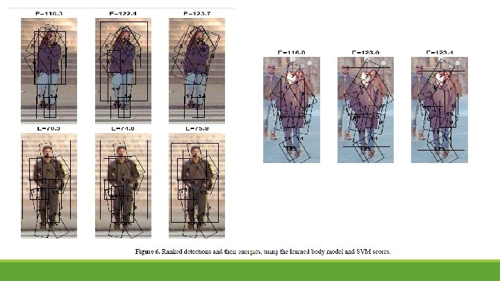
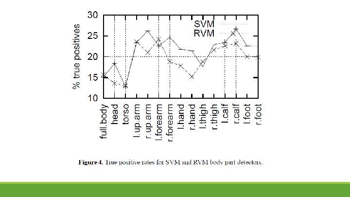
Results- Detection of body parts The RVM classifiers perform only slightly worse than their SVM counterparts, with mean false detection rates of 80. 1% and 78. 5% respectively. The worst results are obtained for the torso and head models, The torso is probably the hardest body part to detect as it is almost entirely shapeless. It is probably best detected indirectly from geometric clues. In contrast, the head is known to contain highly discriminant features, but the training images contain a wide range of poses and significantly more training data

Results- Detection of Body Trees § 100 training examples. §We obtained correct detections rates of 72 % using RVM scores and 83 % using SVM scores. §a majority of the body parts were correctly positioned in only 36 % of the test images for RVM and 55 % for SVM. Second experiment: § 200 training examples. §Detention rate 76% for SVM and 88% for RVM.

References §Finding People by Sampling Ioffe & Forsyth, ICCV 1999 §Probabilistic Methods for Finding People, Ioffe & Forsyth 2001 §Pictorial Structure Models for Object Recognition Felzenszwalb & Huttenlocher, 2000 §Learning to Parse Pictures of People Ronfard, Schmid & Triggs, ECCV 2002