Portfolio Loss Distribution Risky assets in loan portfolio

Portfolio Loss Distribution

Risky assets in loan portfolio • • highly illiquid assets “hold-to-maturity” in the bank’s balance sheet Outstandings The portion of the bank asset that has already been extended to borrowers. Commitment A commitment is an amount the bank has committed to lend. Should the borrower encounter financial difficulties, it would draw on this committed line of credit.

Adjusted exposure and expected loss Let a be the amount of drawn down or usage given default. Outstanding + a commitment, Risky Asset value at later time H, VH (1 -a) commitment, Riskless Adjusted exposure is the risky part of VH. Expected loss = adjusted exposure loss given default probability of default * Normally, practitioners treat the uncertain draw-down rate as a known function of the obligor’s end-of-horizon credit class rating.

Example calculation of expected loss Commitment Outstanding Internal risk rating Maturity Type Unused drawn-down on default (for internal rating = 3) Adjusted exposure on default EDF for internal rating = 3 Loss given default for non-secured asset Expected loss $10, 000 $3, 000 3 1 year Non-secured 65% $8, 250, 000 0. 15% 50% $6, 188

Unexpected loss is the estimated volatility of the potential loss in value of the asset around its expected loss. where Assumptions * The random risk factors contributing to an obligor’s default (resulting in EDF) are statistically independent of the severity of loss (as given by LGD). * The default process is two-state event.

Example on unexpected loss calculation Adjusted exposure $8, 250, 000 EDF 0. 15% s. EDF 3. 87% LGD 50% s. LGD 25% Unexpected loss $178, 511 * The calculated unexpected loss is 2. 16% of the adjusted exposure, while the expected loss is only 0. 075%

Comparison between expected loss and unexpected loss * The higher the recovery rate (lower LGD), the lower is the percentage loss for both EL and UL. * EL increases linearly with decreasing credit quality (with increasing EDF) * UL increases much faster than EL with increasing EDF. Percentage loss per unit of adjusted loss 10% UL EL 5% EDF 10%

Assets with varying terms of maturity * The longer the term to maturity, the greater the variation in asset value due to changes in credit quality. * The two-state default process paradigm inherently ignores the credit losses associated with defaults that occur beyond the analysis horizon. * To mitigate some of the maturity effect, banks commonly adjust a risky asset’s internal credit class rating in accordance with its terms to maturity.

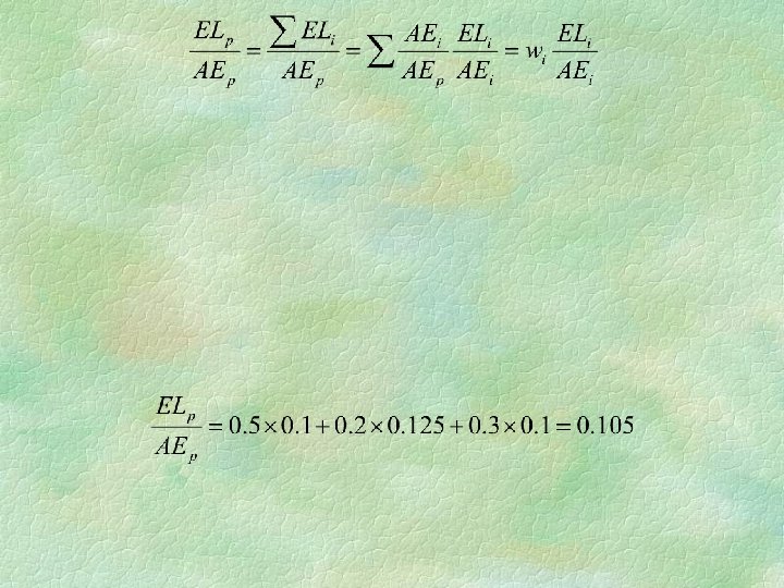
Portfolio expected loss where ELp is the expected loss for the portfolio, AEi is the risky portion of the terminal value of the ith asset to which the bank is exposed in the event of default. We may write where the weights refer to

Portfolio unexpected loss portfolio unexpected loss where and rij is the correlation of default between asset i and asset j. Due to diversification effect, we expect

Risk contribution The risk contribution of a risky asset i to the portfolio unexpected loss is defined to be the incremental risk that the exposure of a single asset contributes to the portfolio’s total risk. and it can be shown that

Undiversifiable risk The risk contribution is a measure of the undiversifiable risk of an asset in the portfolio – the amount of credit risk which cannot be diversified away by placing the asset in the portfolio. To incorporate industry correlation, using i industry a and j industry b

Calculation of EL, UL and RC for a two-asset portfolio r ULp default correlation between the two exposures portfolio expected loss ELp = EL 1 + EL 2 portfolio unexpected loss RC 1 risk contribution from Exposure 1 RC 2 risk contribution from Exposure 2 ELp ULp = RC 1 + RC 2 ULp << UL 1 + UL 2

Fitting of loss distribution The two statistical measures about the credit portfolio are 1. portfolio expected loss; 2. portfolio unexpected loss. 3. At the simplest level, the beta distribution may be chosen to fit the 4. portfolio loss distribution. Reservation A beta distribution with only two degrees of freedom is perhaps insufficient to give an adequate description of the tail events in the loss distribution.

Beta distribution The density function of a beta distribution is Mean and variance f(x, a, b) 1 x

Economic Capital If XT is the random variable for loss and z is the percentage probability (confidence level), what is the quantity v of minimum economic capital EC needed to protect the bank from insolvency at the time horizon T such that Here, z is the desired debt rating of the bank, say, 99. 97% for an AA rating.

frequency of loss ULp XT ELp EC

Capital multiplier Given a desired level of z, what is EC such that Let CM (capital multiplier) be defined by then

Monte Carol simulation of loss distribution of a portfolio 1. Estimate default and losses Assign risk ratings to loss facilities and determine their default probability + Assign LGD and s. LGD 2. Estimate asset correlation between obligors Determine pairwise asset correlation whenever possible OR Assign obligors to industry groupings, then determine industry pair correlation

3. Generate random loss given default Determine stochastic loss given default 4. + Generate correlated default events Correlated Decomposition default + of covariance matrix events + Simulate default point

5. Loss calculation Calculate facility loss for each scenario and obtain portfolio loss 6. Loss distribution Construct simulated portfolio loss distribution

Generation of correlated default events 1. Generate a set of random numbers drawn from a standard normal 2. distribution. 2. Perform a decomposition (Cholesky, SVD or eigenvalue) on the 3. asset correlation matrix to transform the independent set of random 4. numbers (stored in the vectore ) into a set of correlated asset 5. values (stored in the vectore ). Here, the transformation matrix is 6. M, where e = M e. 7. The covariance matrix and M are related by

Calculation of the default point The default point threshold, DP, of the ith obligor can be defined as DP = N-1(EDFi, 0, 1). The criterion of default for the ith obligor is default if no default if

Generate loss given default The LGD is a stochastic variable with an unknown distribution. A typical example may be Recovery rate (%) LGD (%) secured 65 35 21 unsecured 50 50 28 where fi is drawn from a uniform distribution whose range is selected so that the resulting LGD has a standard deviation that is consistent with historical observation.

Calculation of loss Summing all the simulated losses from one single scenario Simulated loss distribution The simulated loss distribution is obtained by repeating the above process sufficiently number of times.

Features of portfolio risk • The variability of default risk within a portfolio is substantial. • The correlation between default risks is generally low. • The default risk itself is dynamic and subject to large fluctuations. • Default risks can be effectively managed through diversification. • Within a well-diversified portfolio, the loss behavior is characterized by lower than expected default credit losses for much of the time, but very large losses which are incurred infrequently.