Portfolio Construction 012609 Portfolio Construction Where does portfolio

Portfolio Construction 01/26/09

Portfolio Construction • Where does portfolio construction fit in the portfolio management process? • What are the foundations of Markowitz’s Mean. Variance Approach (Modern Portfolio Theory)? Twoasset to multiple asset portfolios. • How do we construct optimal portfolios using Mean Variance Optimization? Microsoft Excel Solver. 2

Portfolio Construction • How do we incorporate IPS requirements to determine asset class weights? • What are the assumptions and limitations of the mean-variance approach? • How do we reconcile portfolio construction in practice with Markowitz’s theory? 3

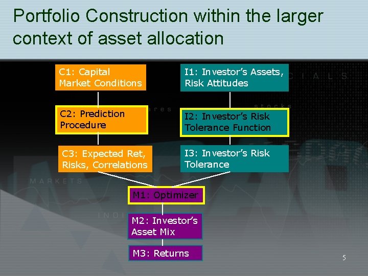
Portfolio Construction within the larger context of asset allocation • IPS provides us with the risk tolerance and return expected by the client • Capital Market Expectations provide us with an understanding of what the returns for each asset class will be 4

Portfolio Construction within the larger context of asset allocation C 1: Capital Market Conditions I 1: Investor’s Assets, Risk Attitudes C 2: Prediction Procedure I 2: Investor’s Risk Tolerance Function C 3: Expected Ret, Risks, Correlations I 3: Investor’s Risk Tolerance M 1: Optimizer M 2: Investor’s Asset Mix M 3: Returns 5

Portfolio Construction within the larger context of asset allocation • Optimization, in general, is constructing the best portfolio for the client based on the client characteristics and CMEs. • When all the steps are performed with careful analysis, the process may be called integrated asset allocation. 6

Mean Variance Optimization • The Mean-Variance Approach, developed by Markowitz in the 1950 s, still serves as the foundation for quantitative approaches to strategic asset allocation. • Mean Variance Optimization (MVO) identifies the portfolios that provide the greatest return for a given level of risk OR that provide the least risk for a given return. 7

Mean Variance Optimization • TO develop an understanding of MVO, we will derive the relationship between risk and return of a portfolio by looking at a series of three portfolios: • One risky asset and one risk-free asset • Two risky assets and one risk-free asset • We will then generalize our findings to portfolios of a larger number of assets. 8

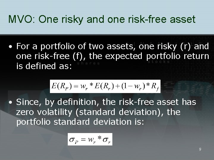
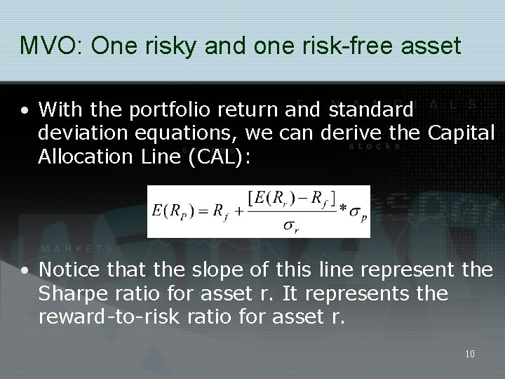
MVO: One risky and one risk-free asset • For a portfolio of two assets, one risky (r) and one risk-free (f), the expected portfolio return is defined as: • Since, by definition, the risk-free asset has zero volatility (standard deviation), the portfolio standard deviation is: 9

MVO: One risky and one risk-free asset • With the portfolio return and standard deviation equations, we can derive the Capital Allocation Line (CAL): • Notice that the slope of this line represent the Sharpe ratio for asset r. It represents the reward-to-risk ratio for asset r. 10

MVO: One risky and one risk-free asset • With one risky and one risk-free asset, an investor can select a portfolio along this CAL based on his risk / return preference. 11

MVO: Two risky assets • With two risky assets (1 and 2), as long as the correlation between the two assets is less than 1, creating a portfolio with the two assets will allow the investor to obtain a greater reward-to-risk ratio than either of the two assets provide. 12

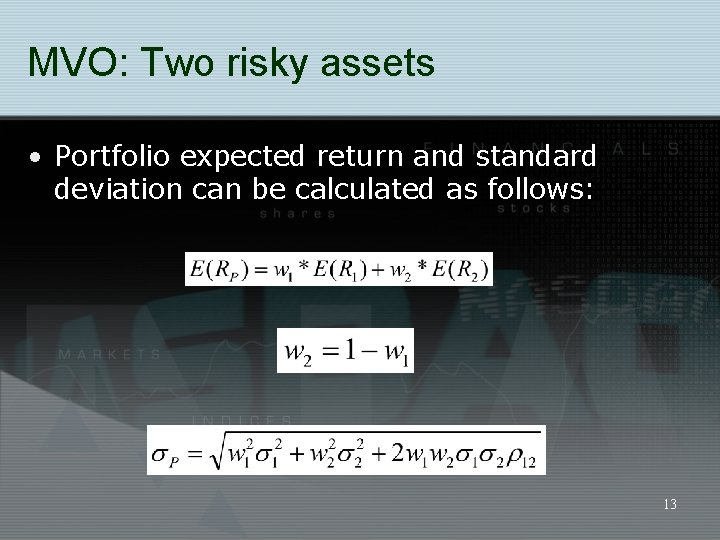
MVO: Two risky assets • Portfolio expected return and standard deviation can be calculated as follows: 13

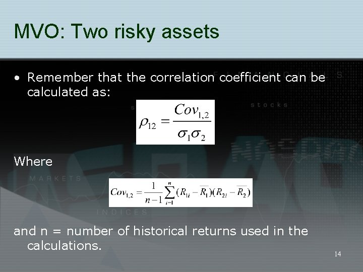
MVO: Two risky assets • Remember that the correlation coefficient can be calculated as: Where and n = number of historical returns used in the calculations. 14

MVO: Two risky assets • These values (as well as asset returns and standard deviations) can be easily calculated on a financial calculator or Excel. 15

MVO: Two risky assets • By altering weights in the two assets, we can construct a minimum-variance frontier (MVF). • The turning point on this MVF represents the global minimum variance (GMV) portfolio. This portfolio has the smallest variance (risk) of all possible combinations of the two assets. • The upper half of the graph represents the efficient frontier. 16

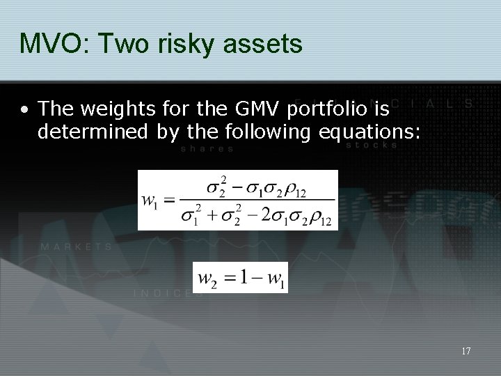
MVO: Two risky assets • The weights for the GMV portfolio is determined by the following equations: 17

MVO: Two risky and one risk-free asset • We know that with one risky asset and the risk-free asset, the portfolio possibilities lie on the CAL. • With two risky assets, the portfolio possibilities lie on the MVF. • Since the slope of the CAL represents the reward-to-risk ratio, an investor will always want to choose the CAL with the greatest slope. 18

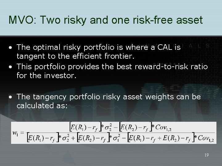
MVO: Two risky and one risk-free asset • The optimal risky portfolio is where a CAL is tangent to the efficient frontier. • This portfolio provides the best reward-to-risk ratio for the investor. • The tangency portfolio risky asset weights can be calculated as: 19

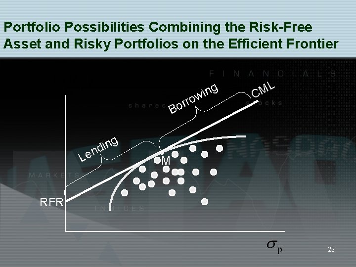
MVO: All risky assets (market) and one risk-free asset • We can generalize our previous results by considering all risky assets and one risk-free asset. The tangency (optimal risky) portfolio is the market portfolio. All investors will hold a combination of the risk-free asset and this market portfolio. • In this context, the CAL is referred to as the Capital Market Line (CML). 20

Investor Risk Tolerance and CML • To attain a higher expected return than is available at the market portfolio (in exchange for accepting higher risk), an investor can borrow at the risk freerate. • Other minimum variance portfolios (on the efficient frontier) are not considered. 21

Portfolio Possibilities Combining the Risk-Free Asset and Risky Portfolios on the Efficient Frontier rr o B g n i nd Le o g n i w L M C M RFR 22

Assumptions / Limitations of Markowitz Portfolio Theory • Investors take a single-period perspective in determining their asset allocation. • Drawback: Investors seldom have a single-period perspective. In a multiple-period horizon, even Treasury bills exhibit variability in returns • Possible Solutions: • Include the “risk-free asset” as a risky asset class. • If investors have a liquidity need, construct an efficient frontier and asset allocation on the funds remaining after the liquidity need is satisfied. 23

Assumptions / Limitations of Markowitz Portfolio Theory • Investors base decisions solely on expected return and risk. These expectations are derived from historical returns. • Drawback: Optimal asset allocations are highly sensitive to small changes in the inputs, especially expected returns. Portfolios may not be well diversified. • Potential solutions: • Conduct sensitivity tests to understand the effect on asset allocation to changes in expected returns. 24

Assumptions / Limitations of Markowitz Portfolio Theory • Investors can borrow and lend at the riskfree rate. • Drawback: Borrowing rates are always higher than lending rates. Certain investors are restricted from purchasing securities on margin. • Potential solutions: • Differential borrowing and lending rates can be easily incorporated into MVO analysis. However, leverage may be practically irrelevant for many investors (liquidity, 25 regulatory restrictions).

Practical Application of MVO • MVO can be used to determine optimal portfolio weights with a certain subset of all investable assets. • An efficient frontier can be constructed with inputs (expected return, standard deviation and correlations) for the selected assets. 26

Practical Application of MVO • MVO can be either unconstrained, in which case we do not place any constraints on the asset weights, or it can be constrained. 27

Practical Application of MVO • Unconstrained Optimization • The simplest optimization places no constraints on asset-class weights except that they add up to 1. • With unconstrained optimization, the asset weights of any minimum variance portfolio is a linear combination of any other two minimum variance portfolios. 28

Practical Application of MVO • Constrained Optimization • The more useful optimization for strategic asset allocation is constrained optimization. • The main constraint is usually a restriction on short sales. 29

Practical Application of MVO • Constrained Optimization • We can determine asset weights using the corner portfolio theorem. This theorem states that the asset weights of any minimum variance portfolio is a linear combination of any two adjacent corner portfolios. • Corner portfolios define a segment of the efficient frontier. 30

Practical Application of MVO • Excel Solver is a powerful tool that can be used to determine optimal portfolio weights for a set of assets. • To use the tool, we need expected returns and standard deviations for our assets as well as a set of constraints that are appropriate for the portfolio. 31

Readings • RB 7 • RB 8 (pgs. 229 -239) • RM 3 (5, 6. 1. 1 – 6. 1. 4) 32