Population parameters Chp 9 Population group of organisms

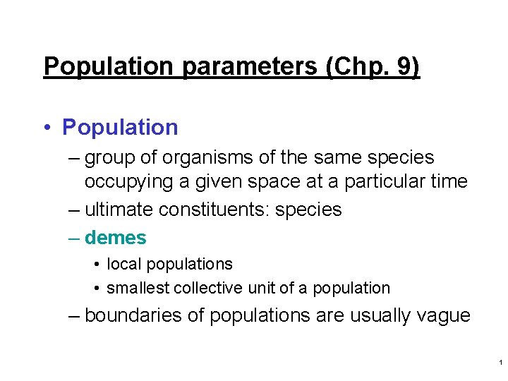
Population parameters (Chp. 9) • Population – group of organisms of the same species occupying a given space at a particular time – ultimate constituents: species – demes • local populations • smallest collective unit of a population – boundaries of populations are usually vague 1

Primary characteristic: density 2

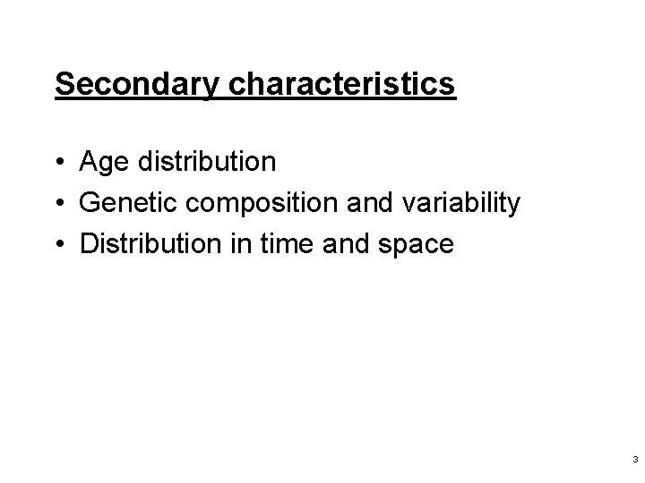
Secondary characteristics • Age distribution • Genetic composition and variability • Distribution in time and space 3

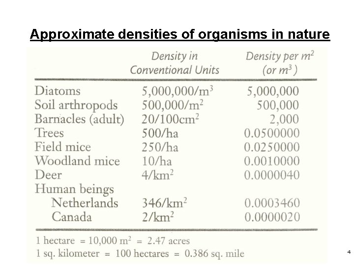
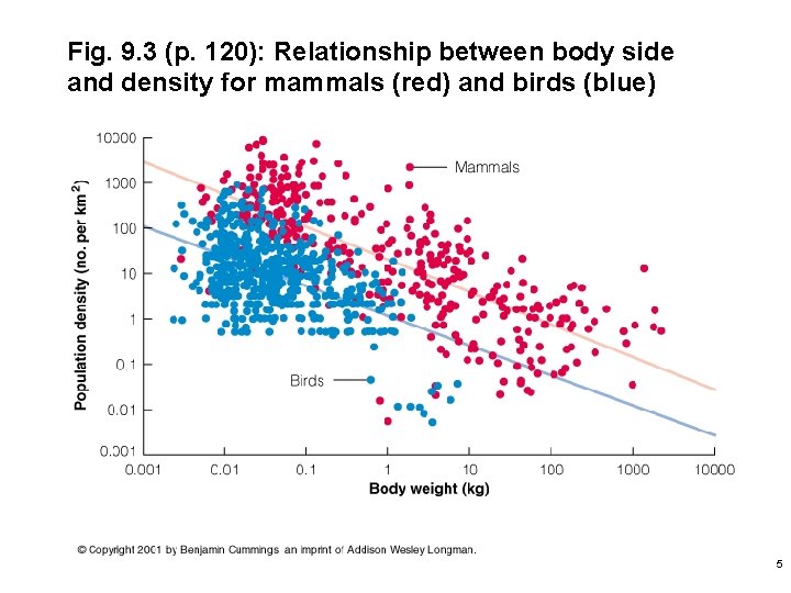
Approximate densities of organisms in nature 4

Fig. 9. 3 (p. 120): Relationship between body side and density for mammals (red) and birds (blue) 5

Measurement of density • Absolute density – estimate of the actual number of individuals in the population • Relative density – collection of samples that represent some relatively constant, but unknown relationship to population size – provides index of abundance, not an estimate of actual density 6

Measurement of absolute density • Total counts – count every individual in the population – census – not possible for many species 7

Measurement of absolute density • Population sampling – count proportion of population and use to estimate size of total population – quadrat sampling • plants • sessile animals – mark-recapture sampling • motile animals 8

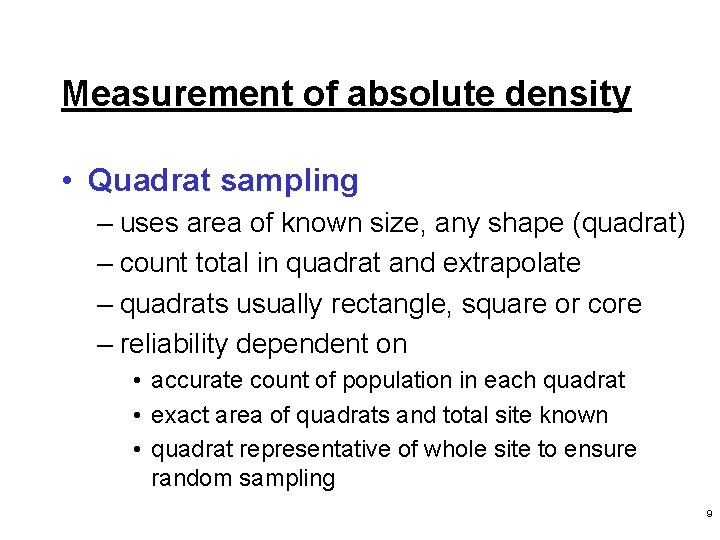
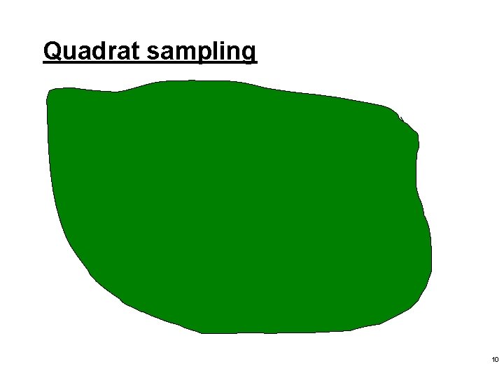
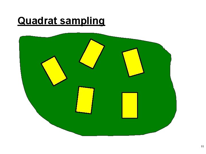
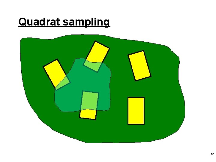
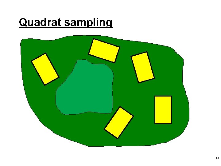
Measurement of absolute density • Quadrat sampling – uses area of known size, any shape (quadrat) – count total in quadrat and extrapolate – quadrats usually rectangle, square or core – reliability dependent on • accurate count of population in each quadrat • exact area of quadrats and total site known • quadrat representative of whole site to ensure random sampling 9

Quadrat sampling 10

Quadrat sampling 11

Quadrat sampling 12

Quadrat sampling 13

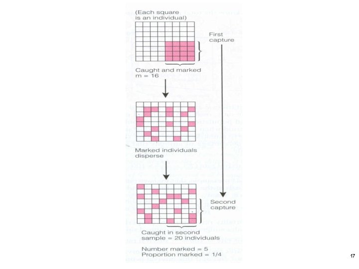
Measurement of absolute density • Mark-recapture sampling – Lincoln-Peterson method – used to estimate • • one-time density of population changes in density over time natality mortality 14

Measurement of absolute density • Mark-recapture sampling – collect, mark and release animals population will consist of both marked and unmarked animals – population size is estimated from determining the proportion of the total population that is marked 15

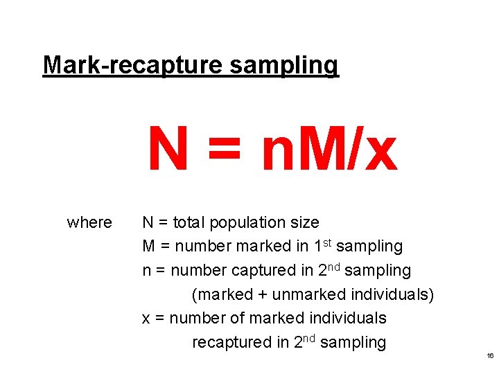
Mark-recapture sampling N = n. M/x where N = total population size M = number marked in 1 st sampling n = number captured in 2 nd sampling (marked + unmarked individuals) x = number of marked individuals recaptured in 2 nd sampling 16

17

Mark-recapture sampling • Assumptions – marked and unmarked individuals are captured randomly (versus trap-happy or trap-shy) – marked individuals are subject to the same mortality as unmarked – marks are not overlooked or lost 18

Measurements of relative density • • • Traps Number of fecal pellets Vocalization frequency Pelt records Questionnaires • • • Aerial photography Roadside counts Feeding capacity Catch per unit effort Number of artifacts 19

Natality: birth rate • Recruitment or addition to population – live birth – hatching – fission – germination – budding 20

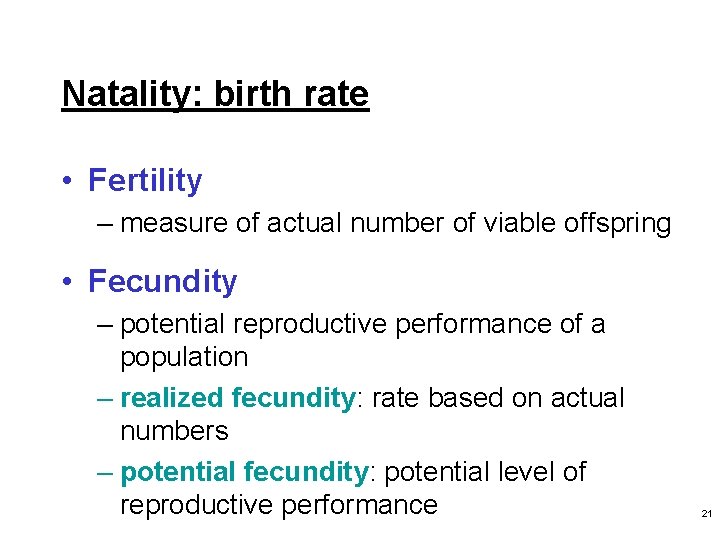
Natality: birth rate • Fertility – measure of actual number of viable offspring • Fecundity – potential reproductive performance of a population – realized fecundity: rate based on actual numbers – potential fecundity: potential level of reproductive performance 21

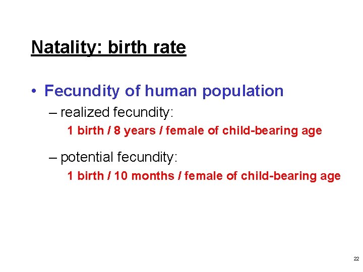
Natality: birth rate • Fecundity of human population – realized fecundity: 1 birth / 8 years / female of child-bearing age – potential fecundity: 1 birth / 10 months / female of child-bearing age 22

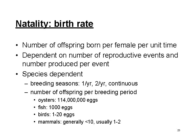
Natality: birth rate • Number of offspring born per female per unit time • Dependent on number of reproductive events and number produced per event • Species dependent – breeding seasons: 1/yr, 2/yr, continuous – number of offspring per breeding period • • oysters: 114, 000 eggs fish: 1000 eggs birds: 1 -20 eggs mammals: generally <10, usually 1 -2 23

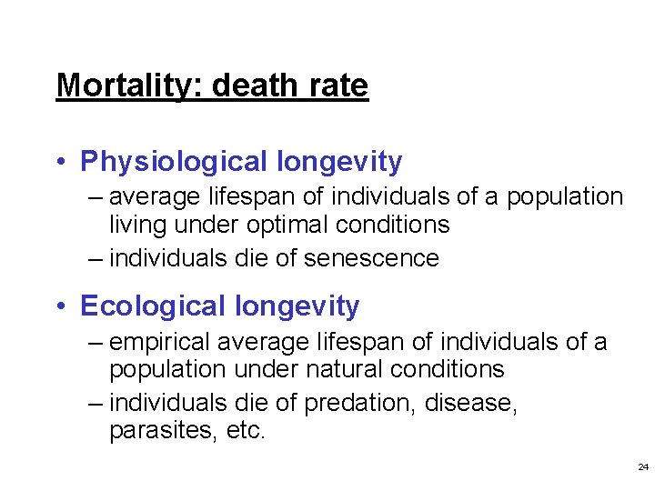
Mortality: death rate • Physiological longevity – average lifespan of individuals of a population living under optimal conditions – individuals die of senescence • Ecological longevity – empirical average lifespan of individuals of a population under natural conditions – individuals die of predation, disease, parasites, etc. 24

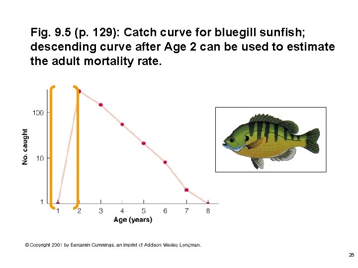
Mortality: death rate • Measurement of mortality rates – direct: mark-recapture experiments over time – indirect: catch curves • survival rates estimated from decreases in relative abundance from age group to age group • survival rate between two years (e. g. , Age 2 -3) = relative abundance of Age 2 / relative abundance of Age 3 25

Fig. 9. 5 (p. 129): Catch curve for bluegill sunfish; descending curve after Age 2 can be used to estimate the adult mortality rate. 26

Limitations on methods used to estimate population density • What constitutes a population of a species? – determining the boundary of the population – distributions along continuums with no distinct boundaries – overlapping populations 27

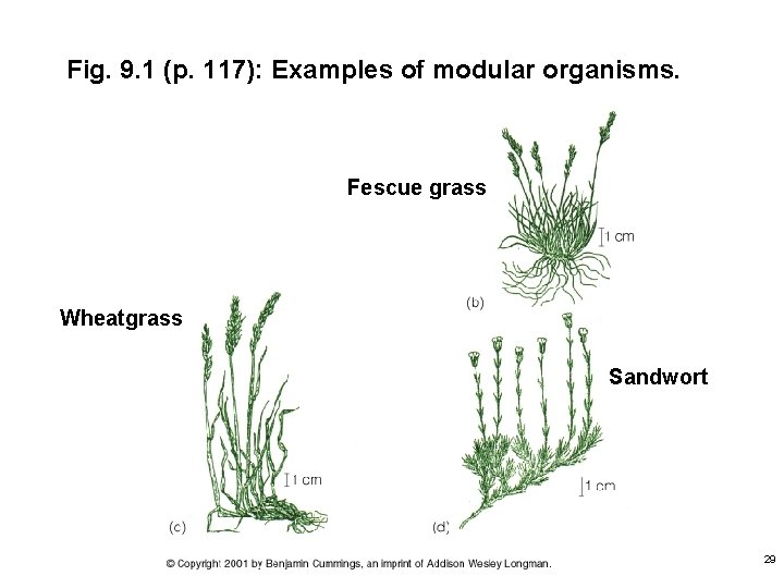
Limitations on methods used to estimate population density • What constitutes an individual in the population? – problem in grasses, colonies of social insects, corals, hybrids, clones, etc. – unitary organisms versus modular organisms – the individual may be the original zygote – biomass or coverage often used to determine density in these populations 28

Fig. 9. 1 (p. 117): Examples of modular organisms. Fescue grass Wheatgrass Sandwort 29

Limitations on methods used to estimate population density • How do differences in community pressures and stresses influence populations? – negative influence on density – positive influence on density 30

Composition of populations • Primary differences – sex ratio • most populations close to 50: 50 • determines reproductive potential of population and many social interactions – age structure • physical size • reproductive rates • disease resistance • social interactions 31

Composition of populations • Secondary differences – color – markings – behavior 32

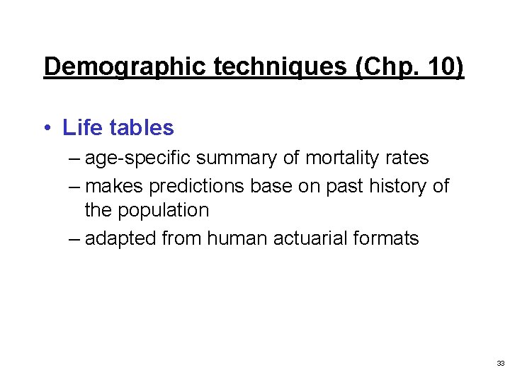
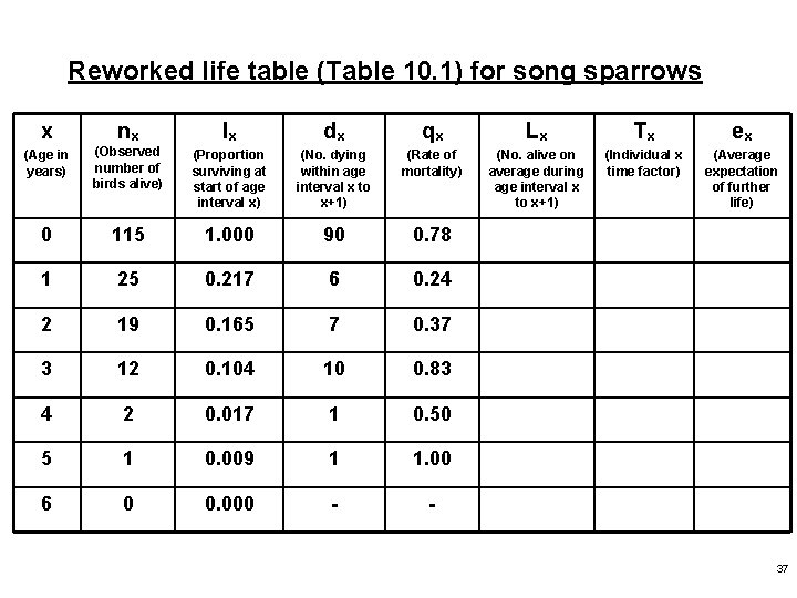
Demographic techniques (Chp. 10) • Life tables – age-specific summary of mortality rates – makes predictions base on past history of the population – adapted from human actuarial formats 33

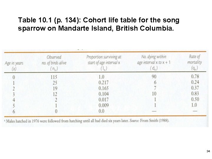
Table 10. 1 (p. 134): Cohort life table for the song sparrow on Mandarte Island, British Columbia. 34

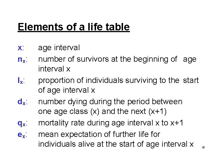
Elements of a life table x: n x: l x: d x: q x: e x: age interval number of survivors at the beginning of age interval x proportion of individuals surviving to the start of age interval x number dying during the period between one age class (x) and the next (x+1) mortality rate during age interval x to x+1 mean expectation of further life for individuals alive at the start of age interval x 35

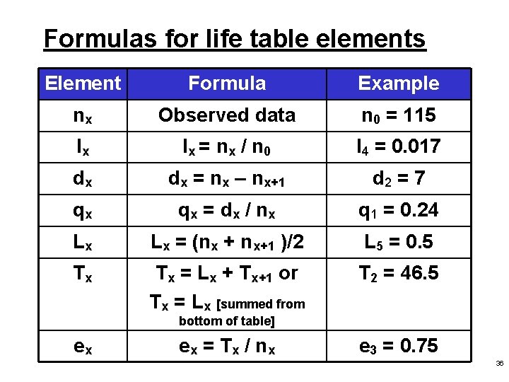
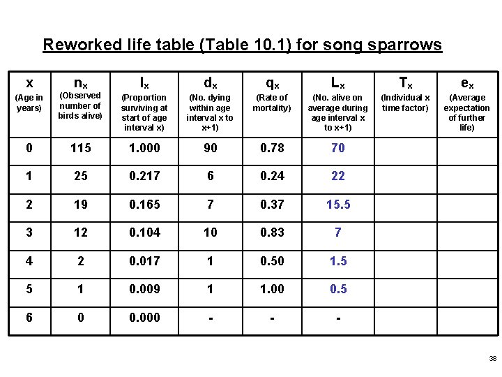
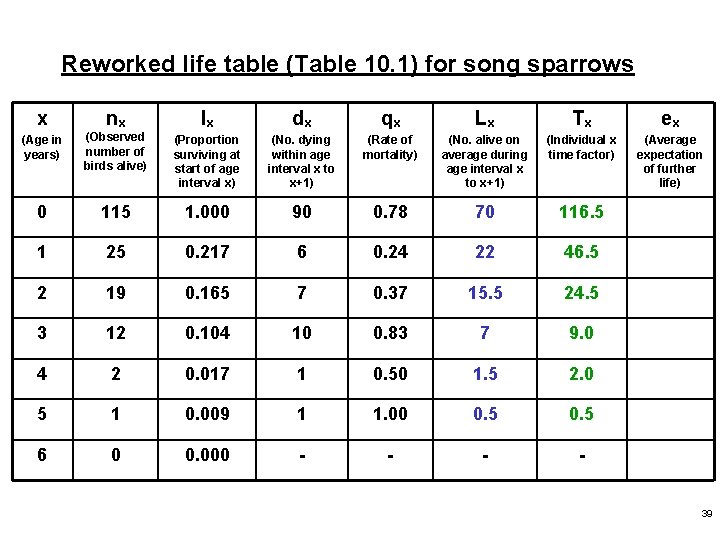
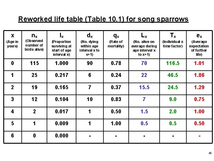
Formulas for life table elements Element Formula Example nx Observed data n 0 = 115 lx lx = n x / n 0 l 4 = 0. 017 dx dx = nx – nx+1 d 2 = 7 qx qx = d x / n x q 1 = 0. 24 Lx Lx = (nx + nx+1 )/2 L 5 = 0. 5 Tx Tx = Lx + Tx+1 or Tx = Lx [summed from T 2 = 46. 5 bottom of table] ex ex = T x / n x e 3 = 0. 75 36

Reworked life table (Table 10. 1) for song sparrows x nx lx dx qx Lx Tx ex (Age in years) (Observed number of birds alive) (Proportion surviving at start of age interval x) (No. dying within age interval x to x+1) (Rate of mortality) (No. alive on average during age interval x to x+1) (Individual x time factor) (Average expectation of further life) 0 115 1. 000 90 0. 78 1 25 0. 217 6 0. 24 2 19 0. 165 7 0. 37 3 12 0. 104 10 0. 83 4 2 0. 017 1 0. 50 5 1 0. 009 1 1. 00 6 0 0. 000 - 37

Reworked life table (Table 10. 1) for song sparrows x nx lx dx qx Lx Tx ex (Age in years) (Observed number of birds alive) (Proportion surviving at start of age interval x) (No. dying within age interval x to x+1) (Rate of mortality) (No. alive on average during age interval x to x+1) (Individual x time factor) (Average expectation of further life) 0 115 1. 000 90 0. 78 70 1 25 0. 217 6 0. 24 22 2 19 0. 165 7 0. 37 15. 5 3 12 0. 104 10 0. 83 7 4 2 0. 017 1 0. 50 1. 5 5 1 0. 009 1 1. 00 0. 5 6 0 0. 000 - - 38

Reworked life table (Table 10. 1) for song sparrows x nx lx dx qx Lx Tx ex (Age in years) (Observed number of birds alive) (Proportion surviving at start of age interval x) (No. dying within age interval x to x+1) (Rate of mortality) (No. alive on average during age interval x to x+1) (Individual x time factor) (Average expectation of further life) 0 115 1. 000 90 0. 78 70 116. 5 1 25 0. 217 6 0. 24 22 46. 5 2 19 0. 165 7 0. 37 15. 5 24. 5 3 12 0. 104 10 0. 83 7 9. 0 4 2 0. 017 1 0. 50 1. 5 2. 0 5 1 0. 009 1 1. 00 0. 5 6 0 0. 000 - - - 39

Reworked life table (Table 10. 1) for song sparrows x nx lx dx qx Lx Tx ex (Age in years) (Observed number of birds alive) (Proportion surviving at start of age interval x) (No. dying within age interval x to x+1) (Rate of mortality) (No. alive on average during age interval x to x+1) (Individual x time factor) (Average expectation of further life) 0 115 1. 000 90 0. 78 70 116. 5 1. 01 1 25 0. 217 6 0. 24 22 46. 5 1. 86 2 19 0. 165 7 0. 37 15. 5 24. 5 1. 29 3 12 0. 104 10 0. 83 7 9. 0 0. 75 4 2 0. 017 1 0. 50 1. 5 2. 0 1. 00 5 1 0. 009 1 1. 00 0. 50 6 0 0. 000 - - 40

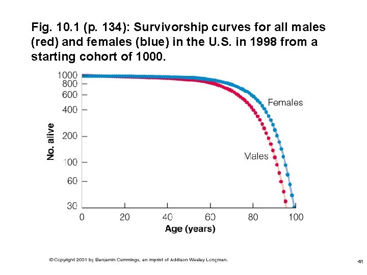
Fig. 10. 1 (p. 134): Survivorship curves for all males (red) and females (blue) in the U. S. in 1998 from a starting cohort of 1000. 41

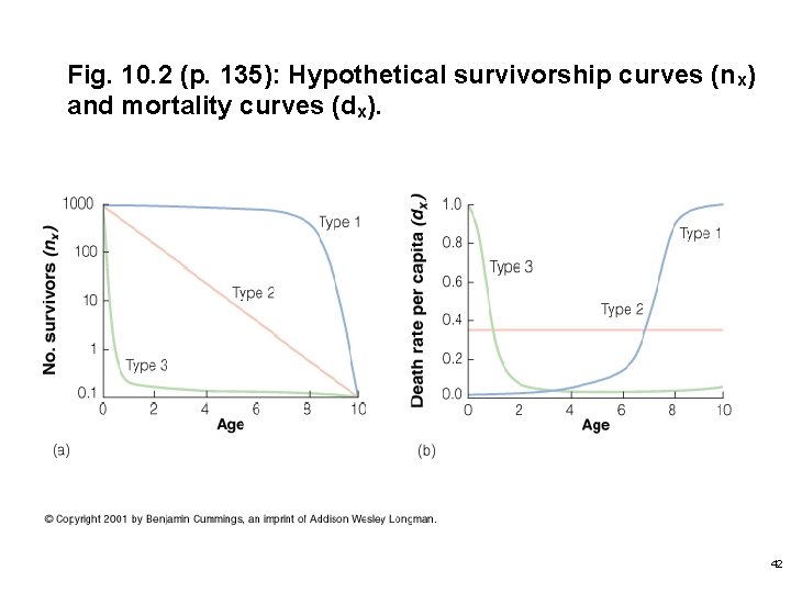
Fig. 10. 2 (p. 135): Hypothetical survivorship curves (nx) and mortality curves (dx). 42

Types of life tables • Static life tables – stationary, time specific, vertical life tables – calculated on basis of a cross-section of the population at a specific time – must be able to determine age of individuals in the population 43

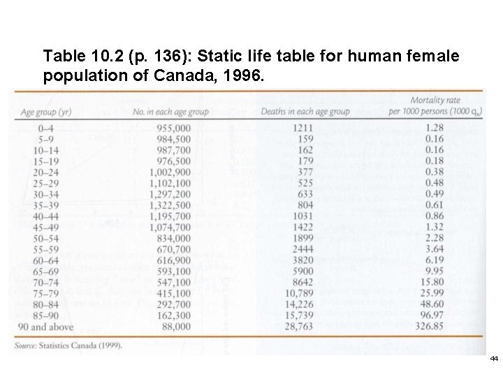
Table 10. 2 (p. 136): Static life table for human female population of Canada, 1996. 44

Types of life tables • Cohort life tables – generational, horizontal life tables – calculated on basis of a cohort of organisms followed from birth through entire life – must be able to track individuals from birth to death 45

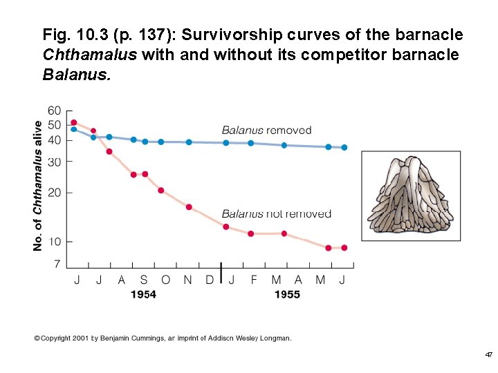
Types of data used for life tables • Survivorship observed directly – lx of cohort is monitored closely over the entire life period – e. g. , Connell’s study of barnacles 46

Fig. 10. 3 (p. 137): Survivorship curves of the barnacle Chthamalus with and without its competitor barnacle Balanus. 47

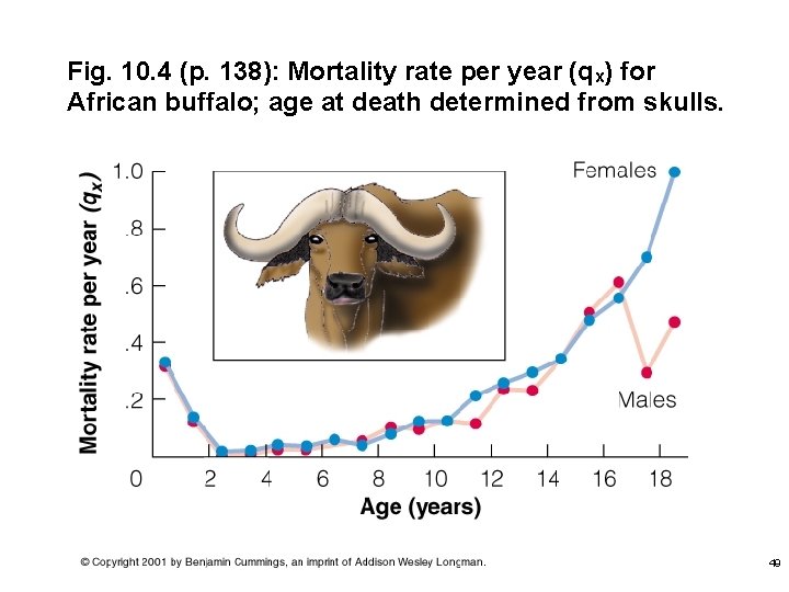
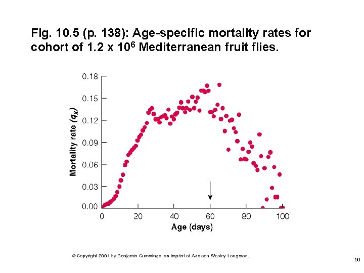
Types of data used for life tables • Age at death observed – assumes population is stable over time and birth and death rates remain constant – e. g. , Sinclair’s study of buffalo (Type I) – e. g. , Carey et al. study of fruit flies (Type III) 48

Fig. 10. 4 (p. 138): Mortality rate per year (qx) for African buffalo; age at death determined from skulls. 49

Fig. 10. 5 (p. 138): Age-specific mortality rates for cohort of 1. 2 x 106 Mediterranean fruit flies. 50

Types of data used for life tables • Population age structure observed directly – requires some way to determine age • annular rings on fish scales • bird plumage • tree rings – not always possible to construct a life table using this kind of data 51

Innate capacity for increasing density • Combines reproduction and life table data • Dependent on environmental conditions – favorable conditions: positive capacity for increase, numbers increase – unfavorable conditions: negative capacity for increase, numbers decrease • In nature, the actual rate of increase varies continuously from positive to negative in response to changes within population – – age distribution social structure genetic composition fluctuations in environmental factors 52

rm: innate capacity for increase • Maximum rate of increase attained at any particular combination of environmental conditions when niche requirements are optimal and other species are entirely excluded from the experiment • Determined only in lab experiments • Changes with different environmental conditions 53

rm: innate capacity for increase • Estimates for rm ra • observed reproductive rate for population r 0 • net reproductive rate • calculated from life table 54

rm: innate capacity for increase • Population innate capacity for increase dependent on – fertility – longevity – speed of development of individual organisms • Natality > mortality population increases • Since natality and mortality rates vary with age structure, quantitative estimates of population growth rates are difficult 55

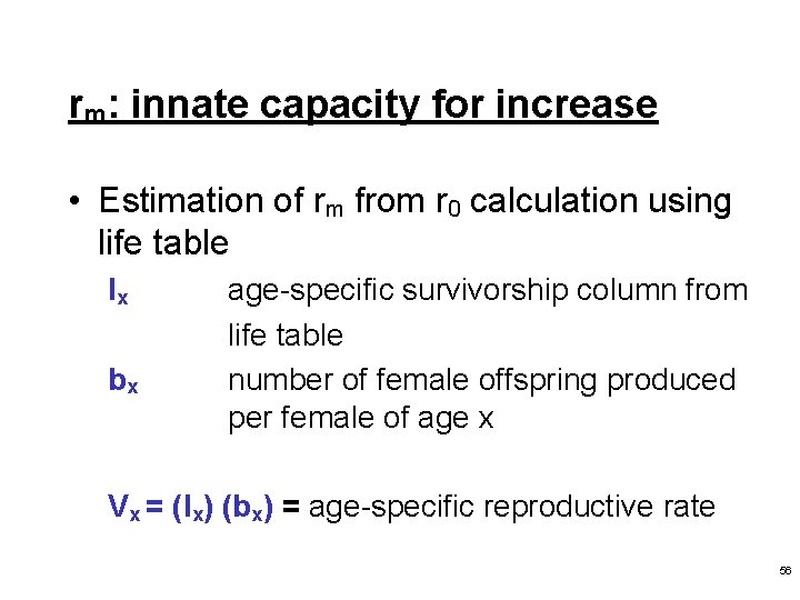
rm: innate capacity for increase • Estimation of rm from r 0 calculation using life table lx bx age-specific survivorship column from life table number of female offspring produced per female of age x Vx = (lx) (bx) = age-specific reproductive rate 56

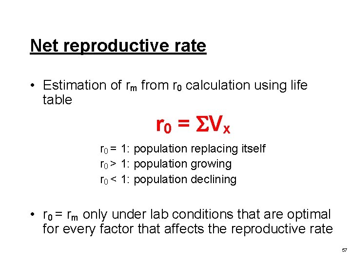
Net reproductive rate • Estimation of rm from r 0 calculation using life table r 0 = Vx r 0 = 1: population replacing itself r 0 > 1: population growing r 0 < 1: population declining • r 0 = rm only under lab conditions that are optimal for every factor that affects the reproductive rate 57