Population Analysis Terminology Estimate Projection Forecast Plan Population

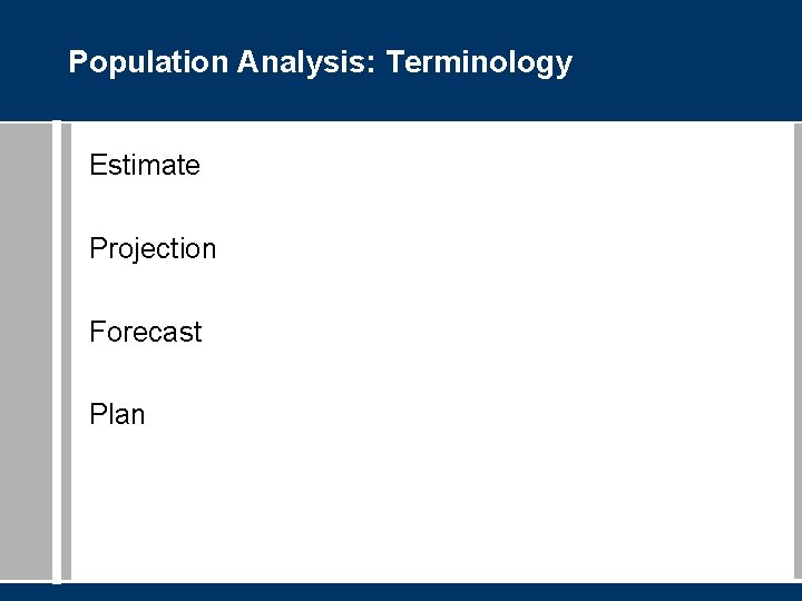
Population Analysis: Terminology Estimate Projection Forecast Plan

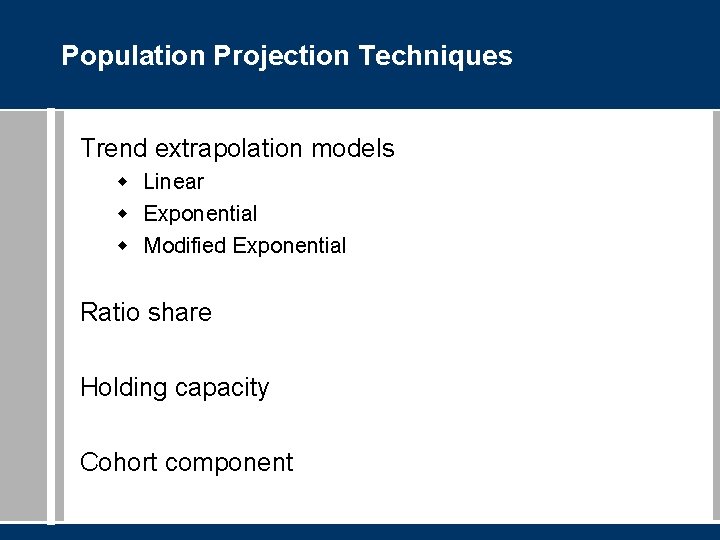
Population Projection Techniques Trend extrapolation models w Linear w Exponential w Modified Exponential Ratio share Holding capacity Cohort component

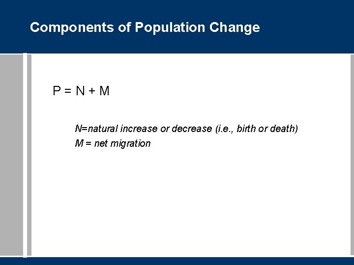
Components of Population Change P=N+M N=natural increase or decrease (i. e. , birth or death) M = net migration

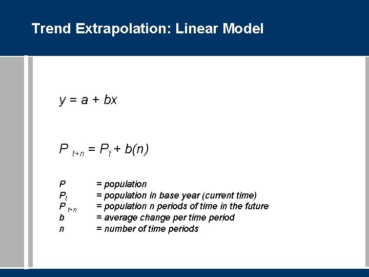
Trend Extrapolation: Linear Model y = a + bx P t+n = Pt + b(n) P Pt P t+n b n = population in base year (current time) = population n periods of time in the future = average change per time period = number of time periods

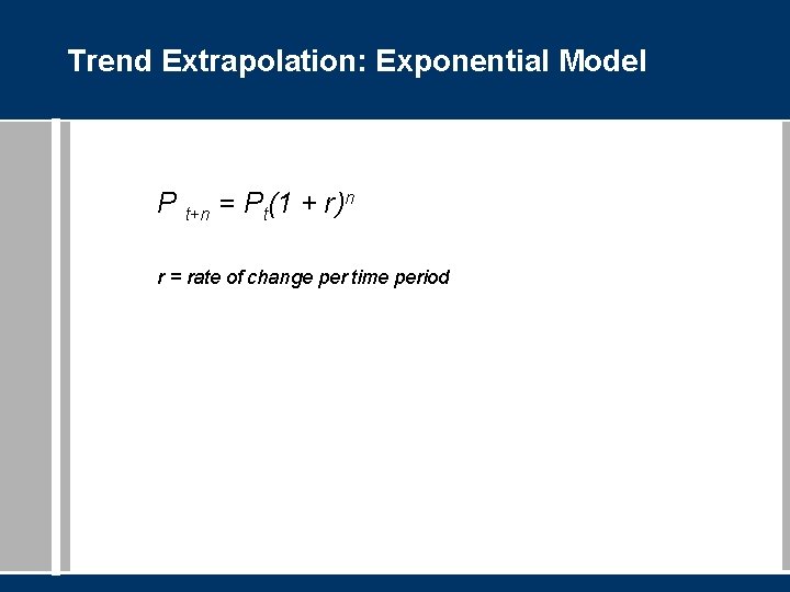
Trend Extrapolation: Exponential Model P t+n = Pt(1 + r)n r = rate of change per time period

Trend Extrapolation: Modified Exponential Model P t+n = K – [(K - Pt) vn] K = maximum capacity v = average portion of unused capacity remaining after each time period

Ratio-Share

Holding Capacity

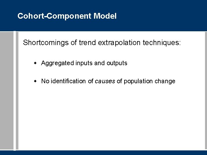
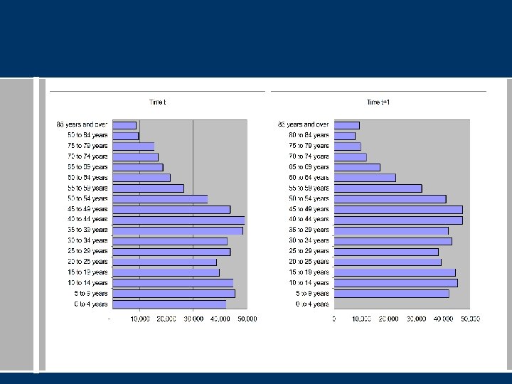
Cohort-Component Model Shortcomings of trend extrapolation techniques: w Aggregated inputs and outputs w No identification of causes of population change

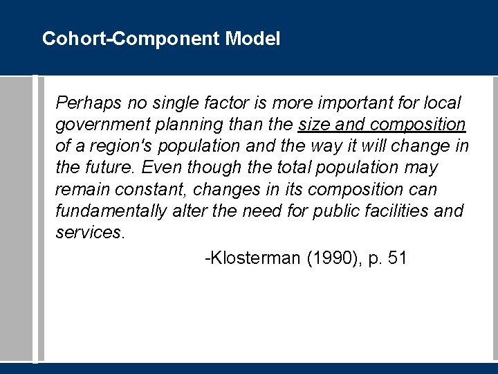
Cohort-Component Model Perhaps no single factor is more important for local government planning than the size and composition of a region's population and the way it will change in the future. Even though the total population may remain constant, changes in its composition can fundamentally alter the need for public facilities and services. -Klosterman (1990), p. 51

Cohort-Component Model Allows for dissagregated view of population change (projects size AND composition) Directly considers causes of population change (death, birth, migration)

Cohort-Component Model Components of Population Change in the Model: w Death (survival rate) w Birth (fertility rate) w Migration (adjust by migration rate)

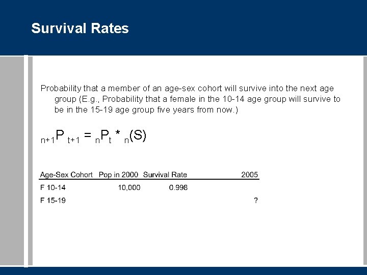
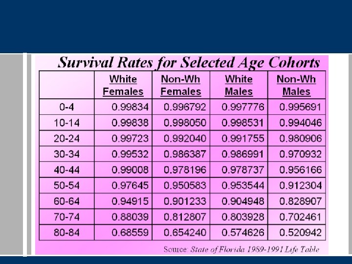
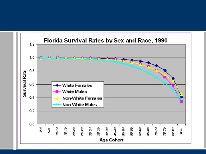
Survival Rates Probability that a member of an age-sex cohort will survive into the next age group (E. g. , Probability that a female in the 10 -14 age group will survive to be in the 15 -19 age group five years from now. ) n+1 P t+1 = n. Pt * n(S)

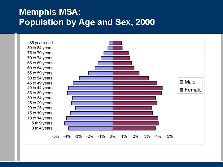
Memphis MSA: Population by Age and Sex, 2000

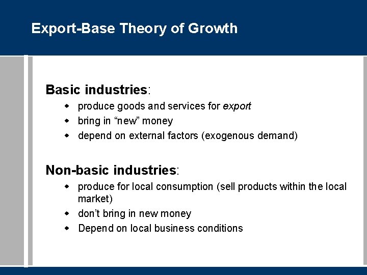
Export-Base Theory of Growth Basic industries: w produce goods and services for export w bring in “new” money w depend on external factors (exogenous demand) Non-basic industries: w produce for local consumption (sell products within the local market) w don’t bring in new money w Depend on local business conditions

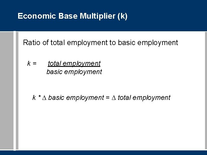
Economic Base Multiplier (k) Ratio of total employment to basic employment k= total employment basic employment k * ∆ basic employment = ∆ total employment

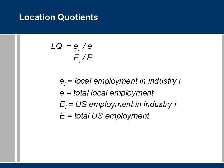
Location Quotients LQ = ei / e Ei / E ei = local employment in industry i e = total local employment Ei = US employment in industry i E = total US employment

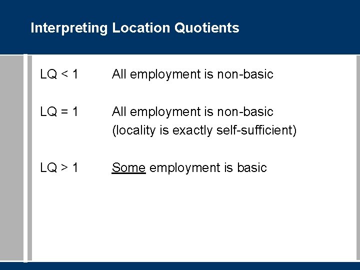
Interpreting Location Quotients LQ < 1 All employment is non-basic LQ = 1 All employment is non-basic (locality is exactly self-sufficient) LQ > 1 Some employment is basic

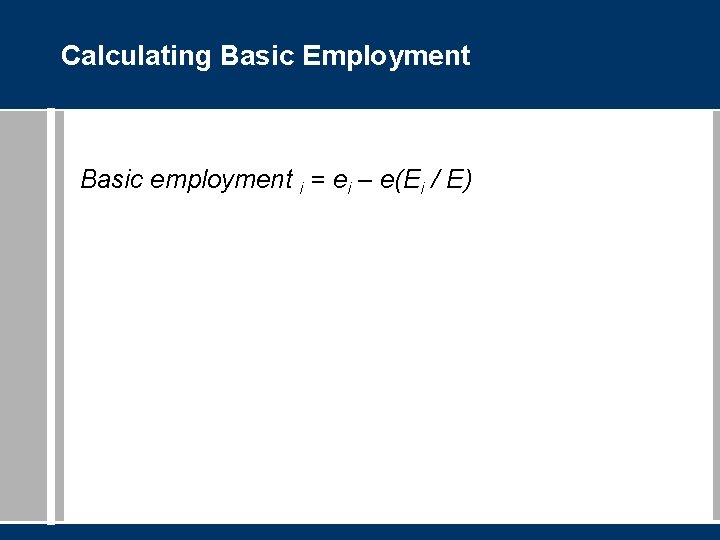
Calculating Basic Employment Basic employment i = ei – e(Ei / E)

Caveats of the LQ Approach Assumptions: 1. Productivity within a specified industry is uniform across all regions 2. Consumption of goods from a given industry is everywhere equal 3. Each industry produces a single homogenous good

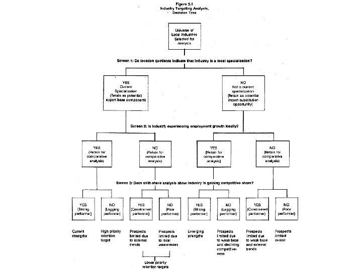
Shift-Share Analysis Partitions local employment growth into 3 components: w National Growth Component w Industrial Mix Component w Competitive Component