Polynomial Time Approximation Scheme PTAS for Euclidian Traveling

Polynomial Time Approximation Scheme (PTAS) for Euclidian Traveling Salesman Problem (TSP) Presented By: Dahan Yakir Sepetnitsky Vitali

Introduction The Traveling Salesman (TSP) problem �Given n points �For each pair {i, j} of distinct points, a cost ci, j �A shortest path is desired �Shortest path = a closed path that �Visits each point exactly once, denote a path like that, as salesman tour �The sum of all distances along the path is minimal (the path have a minimal cost) �This problem is NP-hard

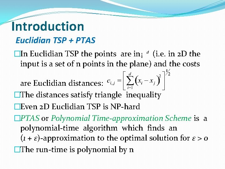
Introduction Euclidian TSP + PTAS �In Euclidian TSP the points are in (i. e. in 2 D the input is a set of n points in the plane) and the costs are Euclidian distances: �The distances satisfy triangle inequality �Even 2 D Euclidian TSP is NP-hard �PTAS or Polynomial Time-approximation Scheme is a polynomial-time algorithm which finds an (1 + ε)-approximation to the optimal solution for ε > 0 �The run-time is polynomial by n

Introduction The algorithm we will present �We will show that Euclidian TSP has a PTAS �The algorithm was given by Sanjeev Arora at 1996 and improved several times through 1996 -1998 �A randomized algorithm will be presented �The PTAS, we will describe, is for points on the plane (d = 2) but there is an extension to an arbitrary d �The algorithm computes an (1 + ε)-approximation to the optimal solution in no(1∕ε) time �The algorithm is based on dynamic programming �The algorithm can be de-randomized, but then the run-time should be increased by a factor of n 4

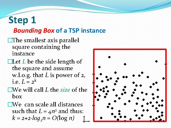
Step 1 Bounding Box of a TSP instance �The smallest axis parallel square containing the instance �Let L be the side length of the square and assume w. l. o. g. that L is power of 2, i. e. L = 2 k �We will call L the size of the box �We can scale all distances such that L = 4 n 2 and thus: k = 2+2∙log 2 n = O(log n)

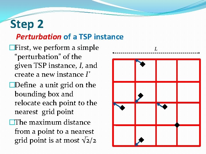
Step 2 Perturbation of a TSP instance �First, we perform a simple “perturbation” of the given TSP instance, I, and create a new instance I’ �Define a unit grid on the bounding box and relocate each point to the nearest grid point �The maximum distance from a point to a nearest grid point is at most √ 2/2 L

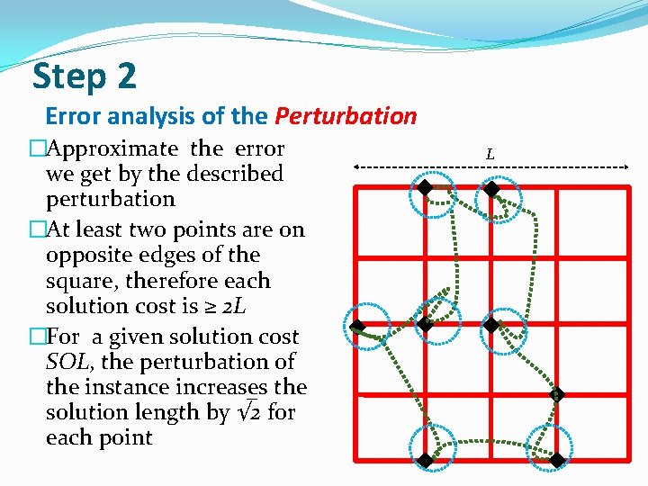
Step 2 Error analysis of the Perturbation �Approximate the error we get by the described perturbation �At least two points are on opposite edges of the square, therefore each solution cost is ≥ 2 L �For a given solution cost SOL, the perturbation of the instance increases the solution length by √ 2 for each point L

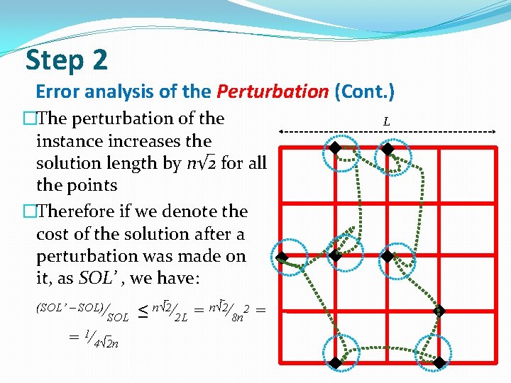
Step 2 Error analysis of the Perturbation (Cont. ) �The perturbation of the instance increases the solution length by n√ 2 for all the points �Therefore if we denote the cost of the solution after a perturbation was made on it, as SOL’ , we have: (SOL’ – SOL)∕ SOL = 1∕ 4√ 2 n ≤ n√ 2∕ 2 L = n√ 2∕ 8 n 2 = L

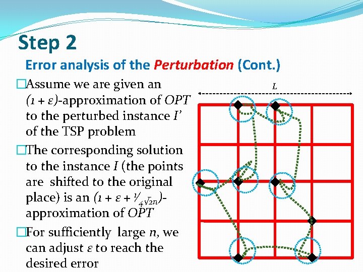
Step 2 Error analysis of the Perturbation (Cont. ) �Assume we are given an (1 + ε)-approximation of OPT to the perturbed instance I’ of the TSP problem �The corresponding solution to the instance I (the points are shifted to the original place) is an (1 + ε + 1∕ 4√ 2 n)approximation of OPT �For sufficiently large n, we can adjust ε to reach the desired error L

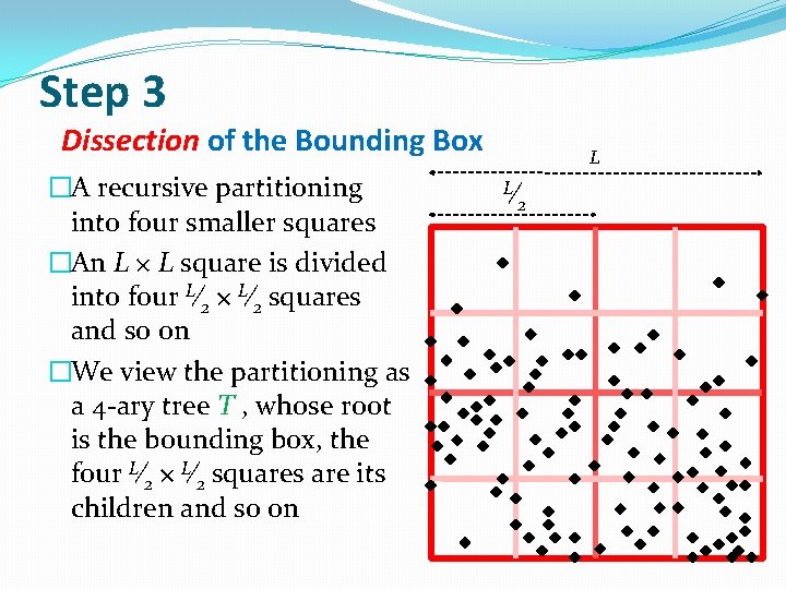
Step 3 Dissection of the Bounding Box �A recursive partitioning into four smaller squares �An L × L square is divided into four L∕ 2 × L∕ 2 squares and so on �We view the partitioning as a 4 -ary tree T , whose root is the bounding box, the four L∕ 2 × L∕ 2 squares are its children and so on L L∕ 2

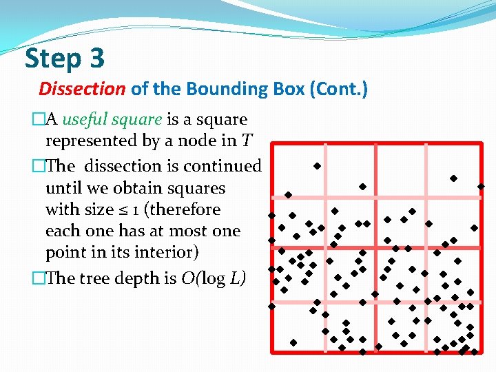
Step 3 Dissection of the Bounding Box (Cont. ) �A useful square is a square represented by a node in T �The dissection is continued until we obtain squares with size ≤ 1 (therefore each one has at most one point in its interior) �The tree depth is O(log L)

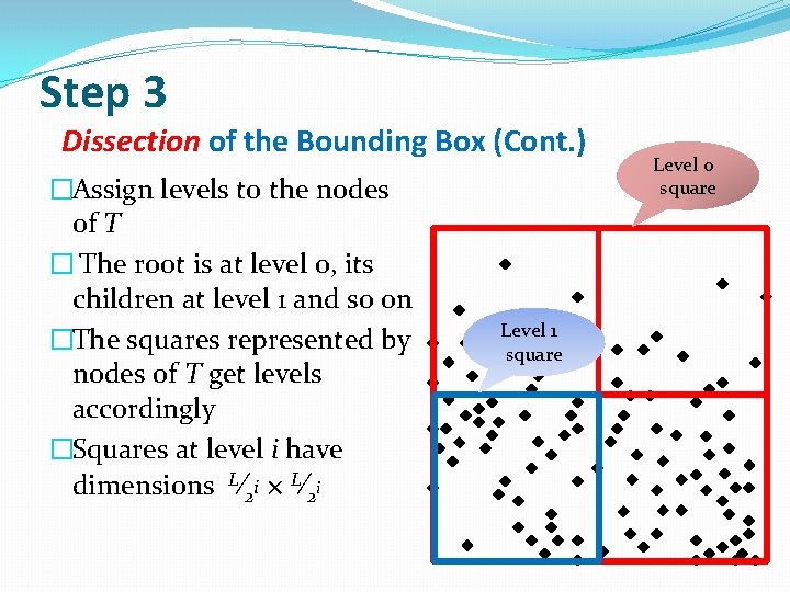
Step 3 Dissection of the Bounding Box (Cont. ) �Assign levels to the nodes of T � The root is at level 0, its children at level 1 and so on �The squares represented by nodes of T get levels accordingly �Squares at level i have dimensions L∕ 2 i × L∕ 2 i Level 1 square Level 0 square

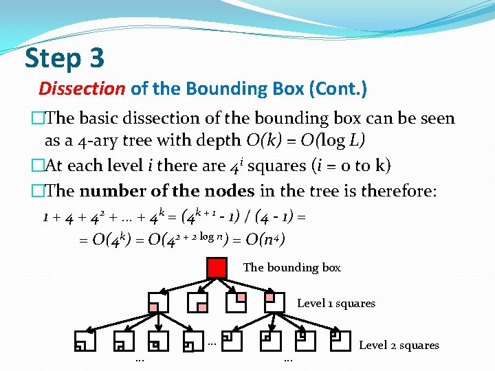
Step 3 Dissection of the Bounding Box (Cont. ) �The basic dissection of the bounding box can be seen as a 4 -ary tree with depth O(k) = O(log L) �At each level i there are 4 i squares (i = 0 to k) �The number of the nodes in the tree is therefore: 1 + 42 + … + 4 k = (4 k + 1 - 1) / (4 - 1) = = O(4 k) = O(42 + 2 log n) = O(n 4) The bounding box Level 1 squares … … … Level 2 squares

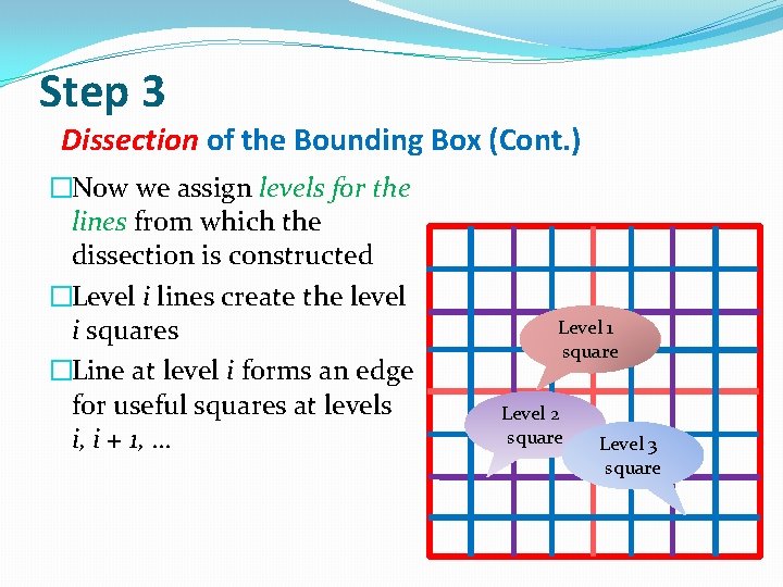
Step 3 Dissection of the Bounding Box (Cont. ) �Now we assign levels for the lines from which the dissection is constructed �Level i lines create the level i squares �Line at level i forms an edge for useful squares at levels i, i + 1, … Level 1 square Level 2 square Level 3 square

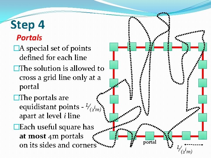
Step 4 Portals �A special set of points defined for each line �The solution is allowed to cross a grid line only at a portal �The portals are equidistant points - L∕(2 im) apart at level i line �Each useful square has at most 4 m portals on its sides and corners portal L∕ i (2 m)

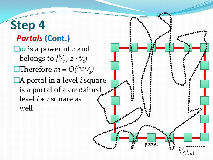
Step 4 Portals (Cont. ) �m is a power of 2 and belongs to [k∕ε , 2 ∙ k∕ε] �Therefore m = O(log n∕ε) �A portal in a level i square is a portal of a contained level i + 1 square as well portal L∕ i (2 m)

Definitions Well behaved tours �A tour τ is well behaved with respect to the basic dissection (WB) if it is a tour through all the n points and any subset of the portals �The tour is allowed to visit portals multiple times �The tour must be non-self-intersecting �A tour τ is well behaved with respect to the basic dissection with limited crossings (WBLC) if it is a well behaved tour (as defined above) and, in addition, it visits each portal at most twice

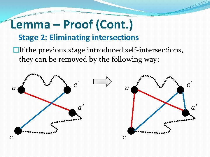
Lemma Well behaved tours (Cont. ) Any well behaved tour τ can be transformed to a WBLC tour, whose length is at most the length of τ Points of the proof: �Given a well behaved tour τ, we will transform it to a WBLC tour τ’ �For each portal in τ, located on line l, which is used more than twice, we will perform a “short-cutting” on the two sides of τ �Then, self intersections (if created) will also be removed from τ’ by short-cutting

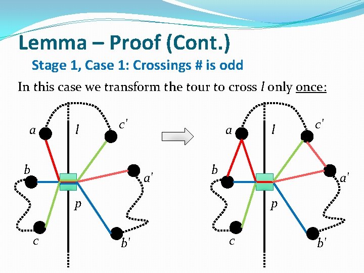
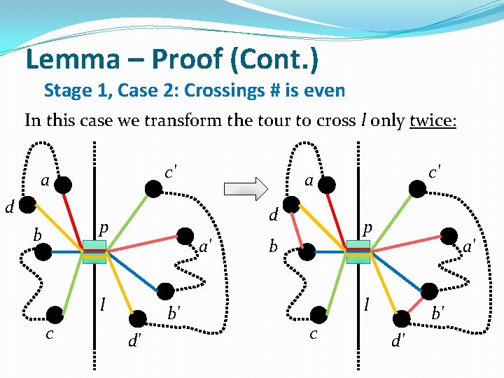
Lemma – Proof Stage 1: Making each portal’s crossings # to be ≤ 2 �Let τ be a well defined tour which crosses a portal p, located on line l, α times (α > 2) �There are two cases: �α is odd �α is even �A “short-cutting” will be performed for each case and make τ cross p at most twice, without increasing its length �The correctness will be guaranteed by triangle inequality

Lemma – Proof (Cont. ) Stage 1, Case 1: Crossings # is odd In this case we transform the tour to cross l only once: a l c' b a a' c' b a' p p c l b' c b'

Lemma – Proof (Cont. ) Stage 1, Case 2: Crossings # is even In this case we transform the tour to cross l only twice: c' a d d p b a' l c b' d' c' a p b a' l c b' d'

Lemma – Proof (Cont. ) Stage 2: Eliminating intersections �If the previous stage introduced self-intersections, they can be removed by the following way: a c' a a’ c c' a’ c

Conclusion The remaining parts of the algorithm �After lemma 1 was proved we know that each WB tour τ can be transformed to a WBLC tour τ’, such that |τ’| ≤ |τ| �We can show that there is a WB tour τ that is short enough, i. e. |τ| ≤ (1 + ε) ∙ OPT �From lemma 1 we know that there exists a WBLC tour τ’ that is short enough too |τ’| ≤ (1 + ε) ∙ OPT �We will obtain all the WBLC tours and take the shortest one τ’’ (the one with minimal sum of distances), therefore |τ’’| ≤ |τ’| |τ’’| ≤ (1 + ε) ∙ OPT

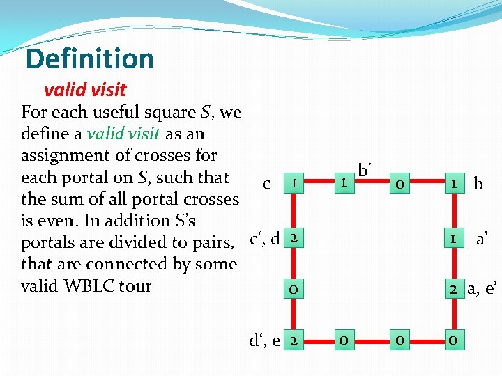
Definition valid visit For each useful square S, we define a valid visit as an assignment of crosses for each portal on S, such that c 1 the sum of all portal crosses is even. In addition S’s portals are divided to pairs, c‘, d 2 that are connected by some valid WBLC tour 0 d‘, e 2 1 b' 0 1 b 1 a' 2 a, e’ 0 0 0

Stage 5 Computing the optimal WBLC The following steps: �We will build a table, that for each square in the dissection, contains the cost of each valid visit. The table will be built up the 4 -ary dissection tree �The calculation uses dynamic programming

Stage 5 Computing the optimal WBLC (Cont. ) �We look only on WBLC tours which means that each portal can be used (= crossed) 0, 1 or 2 times �Denote some WBLC tour by τ �The total number of times, τ can enter or exit a useful square S is at most 8 m �The part of τ inside S, can be viewed as at most 4 m paths, covering all the points inside S �First, we calculate the total number of possibilities to define the number of crossings for each portal on S sides

Stage 5 Computing the optimal WBLC (Cont. ) �The total number of possible assignments is 34 m = 24 m∙log 23 �m in the range [O(log n)∕ε , 2 ∙ O(log n) ∕ε] �Therefore 24 ∙ O(log n)∕ε ∙ (log 3) ≤ 34 m ≤ 28 ∙ O(log n)∕ε ∙ (log 3) ≤ 34 m ≤ n(8 log 3) ∕ε 34 m = n. O(1∕ε) �Among all the possibilities of portals crossings, we retain only those that involve an even sum of crossings (allowing to enter and exit S) �Once we defined the number of crossings for each portal on S sides, not every possible pairing is allowed because of the restriction of the self-intersection �Thus we have n( 4 log 3) ∕ε

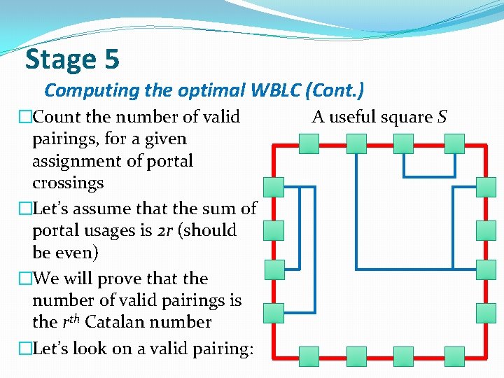
Stage 5 Computing the optimal WBLC (Cont. ) �Count the number of valid pairings, for a given assignment of portal crossings �Let’s assume that the sum of portal usages is 2 r (should be even) �We will prove that the number of valid pairings is the rth Catalan number �Let’s look on a valid pairing: A useful square S

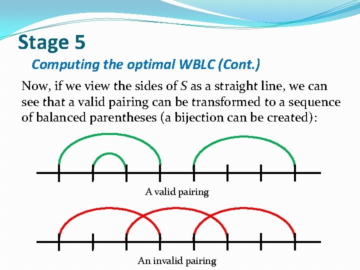
Stage 5 Computing the optimal WBLC (Cont. ) Now, if we view the sides of S as a straight line, we can see that a valid pairing can be transformed to a sequence of balanced parentheses (a bijection can be created): A valid pairing An invalid pairing

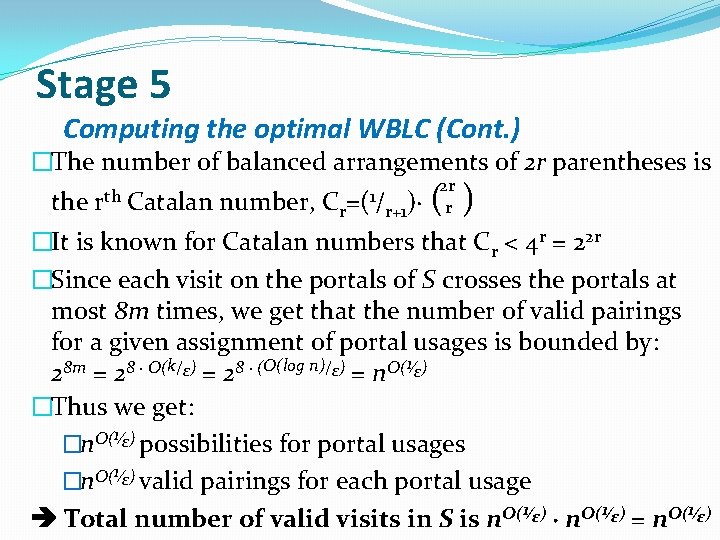
Stage 5 Computing the optimal WBLC (Cont. ) �The number of balanced arrangements of 2 r parentheses is the rth Catalan number, Cr =(1/ r+1)∙ 2 r r ( ) �It is known for Catalan numbers that Cr < 4 r = 22 r �Since each visit on the portals of S crosses the portals at most 8 m times, we get that the number of valid pairings for a given assignment of portal usages is bounded by: 28 m = 28 ∙ O(k/ε) = 28 ∙ (O(log n)/ε) = n. O(1∕ε) �Thus we get: 1 �n. O( ∕ε) possibilities for portal usages 1 �n. O( ∕ε) valid pairings for each portal usage Total number of valid visits in S is n. O(1∕ε) ∙ n. O(1∕ε) = n. O(1∕ε)

Dynamic programming Computing the optimal WBLC: definition of the table �Let’s build the following table in order to compute optimal WBLC cost (for each useful square): Minimum Costs Level 0 Level 1 … Square 1 Square 2 Square 3 Square 4 … valid visit 1 valid visit 2 valid visit 3 … �# of columns = # of squares in the 4 -ary tree = O(n 4) �# of rows = # of valid visits for a square = n. O(1∕ε) �Total # of entries in the table = n 4 ∙ n. O(1∕ε) = n. O(4 + 1∕ε)

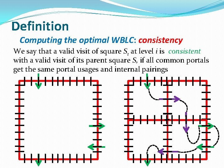
Definition Computing the optimal WBLC: consistency We say that a valid visit of square S 1 at level i is consistent with a valid visit of its parent square S, if all common portals get the same portal usages and internal pairings

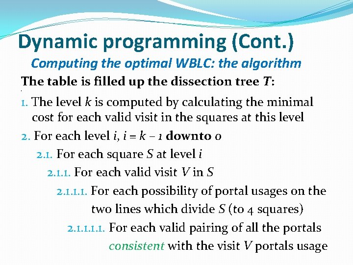
Dynamic programming (Cont. ) Computing the optimal WBLC: the algorithm The table is filled up the dissection tree T: ] 1. The level k is computed by calculating the minimal cost for each valid visit in the squares at this level 2. For each level i, i = k – 1 downto 0 2. 1. For each square S at level i 2. 1. 1. For each valid visit V in S 2. 1. 1. 1. For each possibility of portal usages on the two lines which divide S (to 4 squares) 2. 1. 1. For each valid pairing of all the portals consistent with the visit V portals usage

Dynamic programming (Cont. ) Computing the optimal WBLC: the algorithm (Cont. ) v If the pairing is consistent, it gives rise to valid visits in the four squares internal to S (whose minimal WBLC costs were calculated) 2. 1. 1. 1. Sum the optimal lengths of the appropriate visits in the children squares 2. 1. 1. 1. 2 Compute the minimum cost among the costs for this internal portal usage 2. 1. 1. 2. Compute the minimum cost among the costs for all internal portal usages and store the returned cost in an appropriate entry

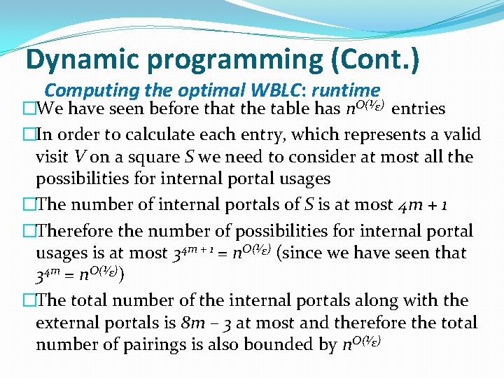
Dynamic programming (Cont. ) Computing the optimal WBLC: runtime 1 �We have seen before that the table has n. O( ∕ε) entries �In order to calculate each entry, which represents a valid visit V on a square S we need to consider at most all the possibilities for internal portal usages �The number of internal portals of S is at most 4 m + 1 �Therefore the number of possibilities for internal portal usages is at most 34 m + 1 = n. O(1∕ε) (since we have seen that 34 m = n. O(1∕ε)) �The total number of the internal portals along with the external portals is 8 m – 3 at most and therefore the total number of pairings is also bounded by n. O(1∕ε)

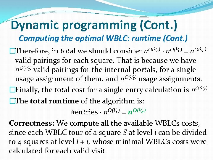
Dynamic programming (Cont. ) Computing the optimal WBLC: runtime (Cont. ) �Therefore, in total we should consider n. O(1∕ε) ∙ n. O(1∕ε) = n. O(1∕ε) valid pairings for each square. That is because we have n. O(1∕ε) valid pairings for the internal portals, for a single usage assignment of them, and n. O(1∕ε) usage assignments. �Finally, the total cost for a single entry calculation is n. O(1∕ε) �The total runtime of the algorithm is: #entries ∙ n. O(1∕ε) = n. O(1∕ε) Correctness: We compute all the available WBLCs costs, since each WBLC tour of a square S at level i can be divided to 4 squares at level i + 1, whose minimal WBLCs costs were calculated for each valid visit

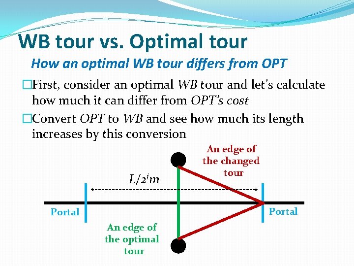
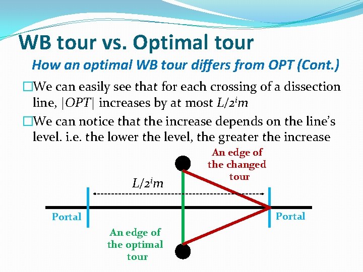
WB tour vs. Optimal tour How an optimal WB tour differs from OPT �First, consider an optimal WB tour and let’s calculate how much it can differ from OPT’s cost �Convert OPT to WB and see how much its length increases by this conversion L/2 im An edge of the changed tour Portal An edge of the optimal tour

WB tour vs. Optimal tour How an optimal WB tour differs from OPT (Cont. ) �We can easily see that for each crossing of a dissection line, |OPT| increases by at most L/2 im �We can notice that the increase depends on the line’s level. i. e. the lower the level, the greater the increase L/2 im An edge of the changed tour Portal An edge of the optimal tour

Is it sufficient? How an optimal WB tour differs from OPT �Is it enough? Is an optimal WB tour always an (1 + ε)-approximation for the optimal TSP solution �The answer is NO!!! �We will show an instance of the Euclidian TSP problem, for which the process of transforming an optimal tour to be WB, increases its length by a fixed constant �Therefore the algorithm will fail if ε is chosen to be below this bound

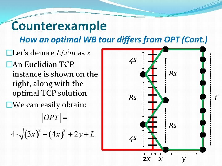
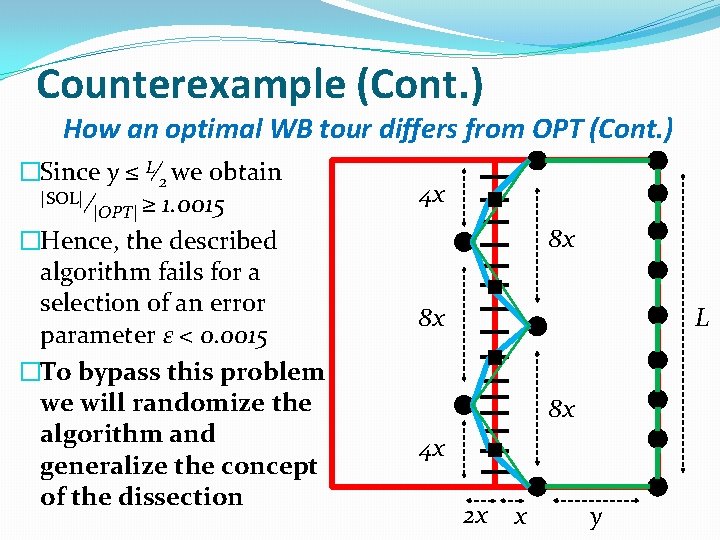
Counterexample How an optimal WB tour differs from OPT (Cont. ) �Let’s denote L/2 im as x �An Euclidian TCP instance is shown on the right, along with the optimal TCP solution �We can easily obtain: 4 x 8 x L 8 x 8 x 4 x 2 x x y

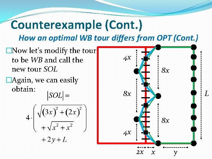
Counterexample (Cont. ) How an optimal WB tour differs from OPT (Cont. ) �Now let’s modify the tour to be WB and call the new tour SOL �Again, we can easily obtain: 4 x 8 x L 8 x 8 x 4 x 2 x x y

Counterexample (Cont. ) How an optimal WB tour differs from OPT (Cont. ) �Since y ≤ L∕ 2 we obtain |SOL| ∕ |OPT| ≥ 1. 0015 �Hence, the described algorithm fails for a selection of an error parameter ε < 0. 0015 �To bypass this problem we will randomize the algorithm and generalize the concept of the dissection 4 x 8 x L 8 x 8 x 4 x 2 x x y

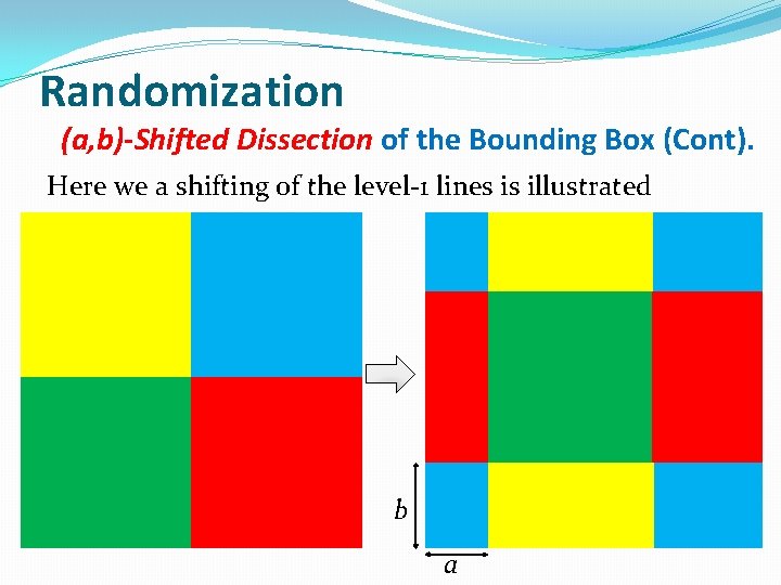
Definition (a, b)-Shifted Dissection of the Bounding Box �Let’s define L 2 different dissections of the bounding box which are shifts of the basic dissection �Choose randomly two integers a and b such that 0 ≤ a, b < L �Shift each vertical line from its original location x to (x + a) mod L �Shift each horizontal line from its original location y to (y + b) mod L � We call the result (a, b)-shifted dissection

Randomization (a, b)-Shifted Dissection of the Bounding Box (Cont). Here we a shifting of the level-1 lines is illustrated b a

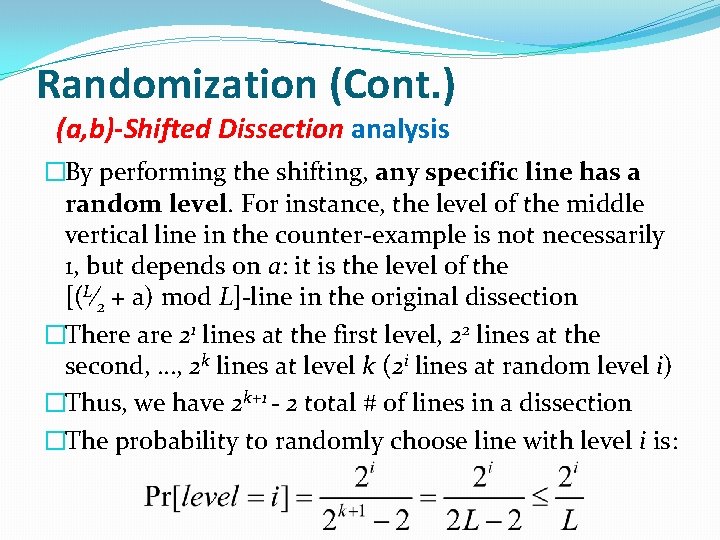
Randomization (Cont. ) (a, b)-Shifted Dissection analysis �By performing the shifting, any specific line has a random level. For instance, the level of the middle vertical line in the counter-example is not necessarily 1, but depends on a: it is the level of the [(L∕ 2 + a) mod L]-line in the original dissection �There are 21 lines at the first level, 22 lines at the second, …, 2 k lines at level k (2 i lines at random level i) �Thus, we have 2 k+1 - 2 total # of lines in a dissection �The probability to randomly choose line with level i is:

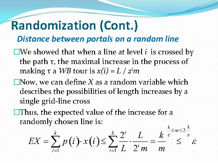
Randomization (Cont. ) Distance between portals on a random line �We showed that when a line at level i is crossed by the path τ, the maximal increase in the process of making τ a WB tour is x(i) = L / 2 im �Now, we can define X as a random variable which describes the possibilities of length increases by a single grid-line cross �Thus, the expected value of the increase for a randomly chosen line is:

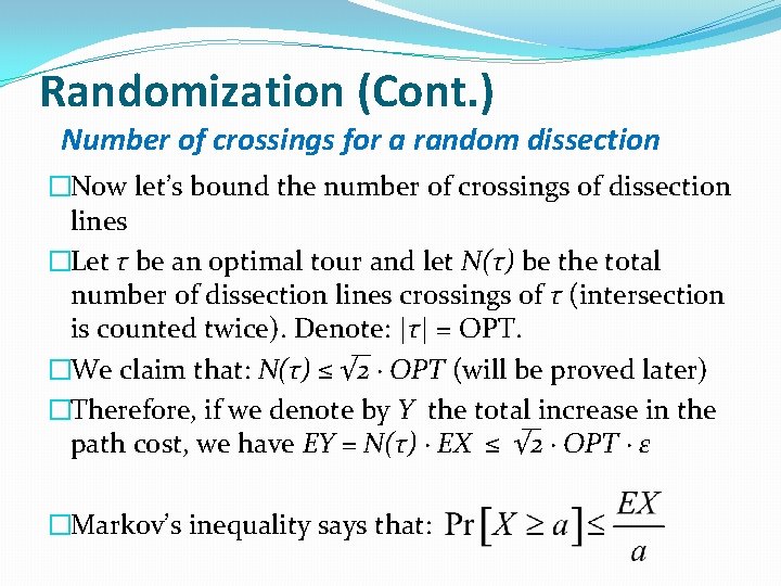
Randomization (Cont. ) Number of crossings for a random dissection �Now let’s bound the number of crossings of dissection lines �Let τ be an optimal tour and let N(τ) be the total number of dissection lines crossings of τ (intersection is counted twice). Denote: |τ| = OPT. �We claim that: N(τ) ≤ √ 2 ∙ OPT (will be proved later) �Therefore, if we denote by Y the total increase in the path cost, we have EY = N(τ) ∙ EX ≤ √ 2 ∙ OPT ∙ ε �Markov’s inequality says that:

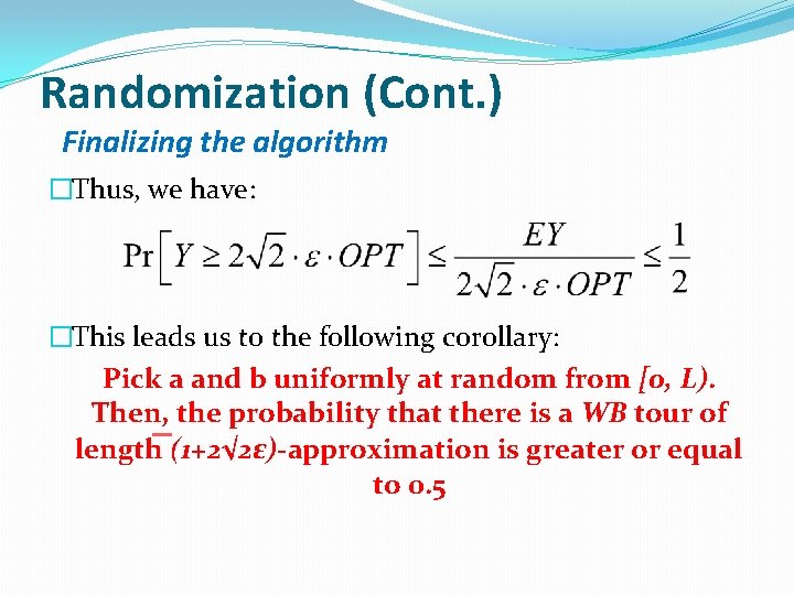
Randomization (Cont. ) Finalizing the algorithm �Thus, we have: �This leads us to the following corollary: Pick a and b uniformly at random from [0, L). Then, the probability that there is a WB tour of length (1+2√ 2ε)-approximation is greater or equal to 0. 5

Randomization (Cont. ) Finalizing the algorithm (Cont. ) Three remarks: �The 2√ 2 prefix can be removed by updating ε to ε’ > 0 which can be calculated by solving the equation 2√ 2ε’ = ε �We can reduce the probability that the total increase in length is to high, by repeating the procedure for c different (a, b)-shifted dissections and choosing the shortest tour �We can derandomize the algorithm by trying all the possible L 4 = O(n 4) dissection and, again, choosing the shortest tour

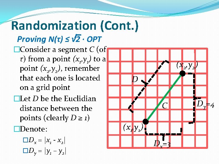
Randomization (Cont. ) Proving N(τ) ≤ √ 2 ∙ OPT �Consider a segment C (of τ) from a point (x 1, y 1) to a point (x 2, y 2), remember that each one is located on a grid point �Let D be the Euclidian distance between the points (clearly D ≥ 1) �Denote: �Dx = |x 1 - x 2| �Dy = |y 1 – y 2| (x 2, y 2) D C (x 1, y 1) Dx=3 Dy=4

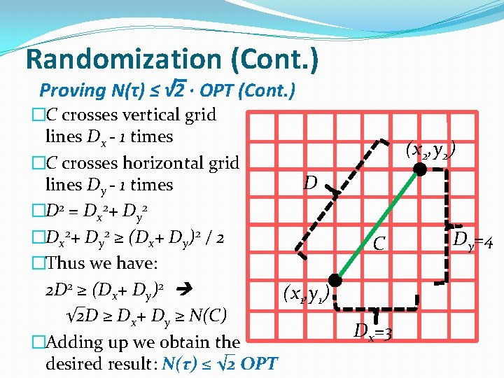
Randomization (Cont. ) Proving N(τ) ≤ √ 2 ∙ OPT (Cont. ) �C crosses vertical grid lines Dx - 1 times �C crosses horizontal grid D lines Dy - 1 times �D 2 = Dx 2+ Dy 2 �Dx 2+ Dy 2 ≥ (Dx+ Dy)2 / 2 �Thus we have: 2 D 2 ≥ (Dx+ Dy)2 (x 1, y 1) √ 2 D ≥ Dx+ Dy ≥ N(C) �Adding up we obtain the desired result: N(τ) ≤ √ 2 OPT (x 2, y 2) C Dx=3 Dy=4

Summary PTAS for Euclidian TSP (in R 2) Given a TSP instance, perform: 1. Find the bounding box 2. Perturbation of the instance 3. Create an (a, b)-shifted dissection of the bounding box for some randomly chosen integers 0 ≤ a, b < L 4. Calculate an optimal WBLC tour τ, using dynamic programming 5. With probability of at least 1∕ 2 , τ is an (1 + ε)approximation to the optimal solution 6. Repeat 3 -5 until the required probability is obtained

References �V. V. Vazirani, Approximation Algorithms, Springer, 2001. �Sanjeev Arora, Polynomial-time Approximation Schemes for Euclidean TSP and other Geometric Problems, Journal of the ACM 45(5) 753– 782, 1998.