POLYNOMIAL APPROACH TO DISTRIBUTIONS VIA SAMPLING Papatsouma Ioanna

POLYNOMIAL APPROACH TO DISTRIBUTIONS VIA SAMPLING Papatsouma Ioanna Department of Mathematics Aristotle University of Thessaloniki Greece

AIM & OBJECTIVES Aim: Define distribution models via sampling, connected with socio-economic, political, medical or biological issues. Objectives: • Approach all kind of distributions (symmetric, descending, decreasing) using Coefficient of Variation • Investigate what happens when the rv X does not take values in an infinite set, but the range becomes finite • Verify and validate the distribution models found

Distributions are like a puzzle… Symmetric Increasing Descending Polynomial approach …and the missing piece was found!

SYMMETRIC DISTRIBUTIONS a = 0

SYMMETRIC DISTRIBUTIONS: THE CASE OF SINE DISTRIBUTIONS
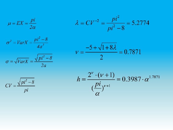

The pdf is:

INCREASING DISTRIBUTIONS

DESCENDING DISTRIBUTIONS TYPE I

DESCENDING DISTRIBUTIONS TYPE II

NEGATIVE EXPONENTIAL DISTRIBUTION Suppose that the rv X has a descending exponential distribution. The corresponding pdf is given by the expression:

So, the above function is the pdf of rv X that take values in [0, b].

TRUNCATED NEGATIVE EXPONENTIAL DISTRIBUTION

EXAMPLES 1. In an online educational experiment, n = 120 students are trying to find each one separately the answer in question «When was the Parthenon built in Greece? » . Χ=time (sec) it took each student to find the correct answer using a web search engine.
 37. 5 8 [75, 150) 112.")
Classes Class centers xi Frequencies ni [0, 75) 37. 5 8 [75, 150) 112. 5 15 [150, 225) 187. 5 24 [225, 300) 262. 5 26 [300, 375) 337. 5 23 [375, 450) 412. 5 15 [450, 525] 487. 5 9 Total 120

30 26 24 25 23 20 15 15 10 15 9 8 5 0 37. 5 112. 5 187. 5 262. 5 337. 5 412. 5 487. 5
 37. 5 8 -3 -24 72 [75,")
Classes xi ni xi ΄2 [0, 75) 37. 5 8 -3 -24 72 [75, 150) 112. 5 15 -2 -30 60 [150, 225) 187. 5 24 -1 -24 24 [225, 300) m=262. 5 26 0 0 0 [300, 375) 337. 5 23 1 23 23 [375, 450) 412. 5 15 2 30 60 [450, 525] 487. 5 9 3 27 81 T 1=2 T 2=320 Total 120
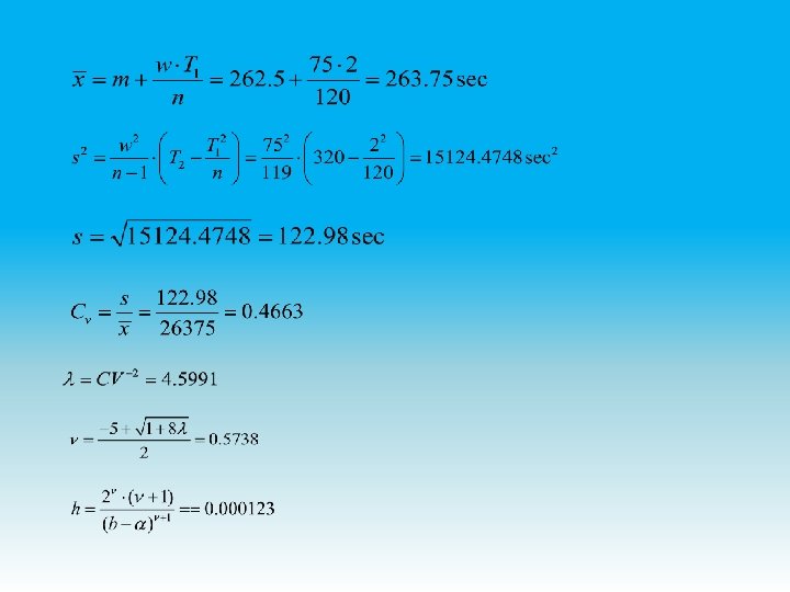

μ σ2 σ CV λ ν h 263. 75 15124. 4748 122. 98 0. 4663 4. 5991 0. 5738 0. 000123 The polynomial pdf is: and the corresponding cdf is:

The trigonometric pdf is: and the corresponding cdf is:
 Φ(x) f(x) F(x) |Φ(x)-F(x)| [0, 75) 0. 0495 0. 0697 0. 0202")
x φ(x) Φ(x) f(x) F(x) |Φ(x)-F(x)| [0, 75) 0. 0495 0. 0697 0. 0202 [75, 150) 0. 1387 0. 1882 0. 1377 0. 2074 0. 0192 [150, 225) 0. 2005 0. 3887 0. 1852 0. 3926 0. 0039 [225, 300) 0. 2226 0. 6113 0. 2148 0. 6074 0. 0039 [300, 375) 0. 2005 0. 8118 0. 1852 0. 7926 0. 0192 [375, 450) 0. 1387 0. 9505 0. 1377 0. 9303 0. 0202 [450, 525] 0. 0495 1 0. 0697 1 0
 = Φ(x) H 1: F(x) ≠ Φ(x)")
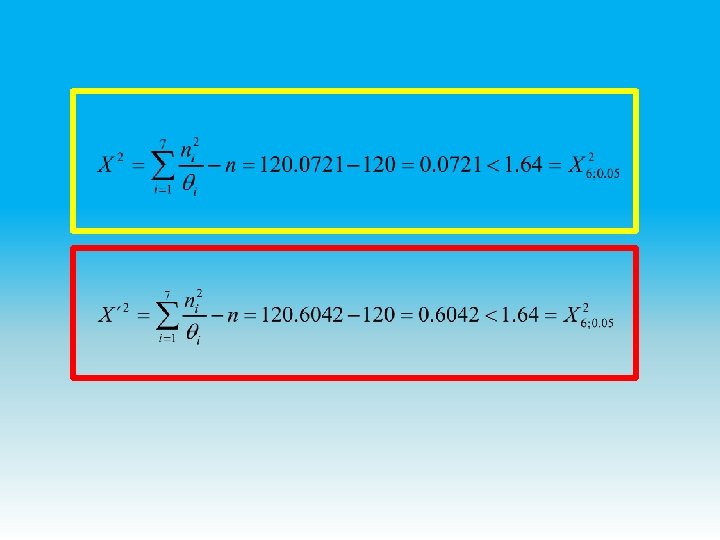
Testing the following hypotheses: H 0: F(x) = Φ(x) H 1: F(x) ≠ Φ(x) It follows that: D 7, 7 = max |Φ(x)-F(x)| = 0. 0202 Kolmogorov-Smirnov table gives the critical value c: D 7, 7; 0. 05 = 0. 7143
 θi ni 2/θi f(x) θi΄ ni 2/θi΄ [0, 75) 8 0.")
x ni φ(x) θi ni 2/θi f(x) θi΄ ni 2/θi΄ [0, 75) 8 0. 0495 5. 9 10. 8474 0. 0697 8. 4 7. 6190 [75, 150) 15 0. 1387 16. 6 13. 5542 0. 1377 16. 5 13. 6364 [150, 225) 24 0. 2005 24. 0000 0. 1852 22. 2 25. 9459 [225, 300) 26 0. 2226 26. 7 25. 3184 0. 2148 25. 8 26. 2016 [300, 375) 23 0. 2005 24. 1 21. 9502 0. 1852 22. 2 25. 9459 [375, 450) 15 0. 1387 16. 6 13. 5545 0. 1377 16. 5 13. 6364 [450, 525] 9 0. 0495 5. 9 10. 8474 0. 0697 8. 4 7. 6190

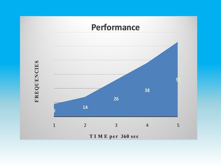
2. In an online educational experiment, a very difficult question was given to n = 140 students and maximum time to answer Xmax = 1800 seconds. Students who exhausted all time without answering, were considered to have performance Χ=1800 seconds.
 180 9 9 -2 -18")
Classes Class Frequencies centers xi ni [0 - 360) 180 9 9 -2 -18 32 6. 9 11. 739 [360 - 720) 540 14 23 -1 -14 14 18. 3 10. 710 [720 – 1080) 900=m 26 49 0 0 0 28. 6 23. 636 [1080 – 1440) 1260 38 87 1 38 38 38. 4 37. 604 [1440 – 1800] 1620 53 140 2 106 212 T 1=114 T 2=300 47. 8 n=140 58. 766 Χ 2=2. 2455 n=140 Νi θi Χ 2

The pdf is: and the corresponding cdf is:

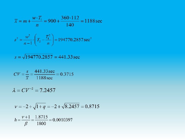
3. In an online educational experiment, a very easy question was given to n = 160 students and maximum time to answer Xmax = 900 seconds.
 270 41 [360 –")
Classes Class centers xi 90 Frequencies ni [180 – 360) 270 41 [360 – 540) 450 30 [540 – 720) 630 15 [720 – 900] 810 10 n=160 [0 – 180) Total 64
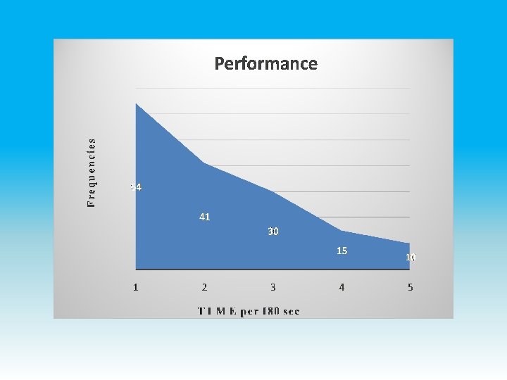
 90")
Classes Νi θi Χ 2 Class Frequencies centers xi ni [0 – 180) 90 64 64 -2 -128 256 66. 3 0. 080 [180 – 360) 270 41 105 -1 -41 41 46. 7 0. 696 [360 – 540) m=450 30 135 0 0 0 29. 2 0. 022 [540 – 720) 630 15 150 1 15 15 14. 4 2. 912 [720 – 900] 810 10 160 2 20 40 3. 4 Consump tion 160 Χ 2=3. 71 Total n=160 T 1=-134 T 2=352

TYPE I The pdf is: and the cdf is:

TYPE II The pdf is: and the cdf is: Both methods show that data are adapted to theoritical frequencies, since Χ 2 =3. 71 < 9. 488 (Type I) and Χ 2 =4. 0214 < 9. 488 (Type II).

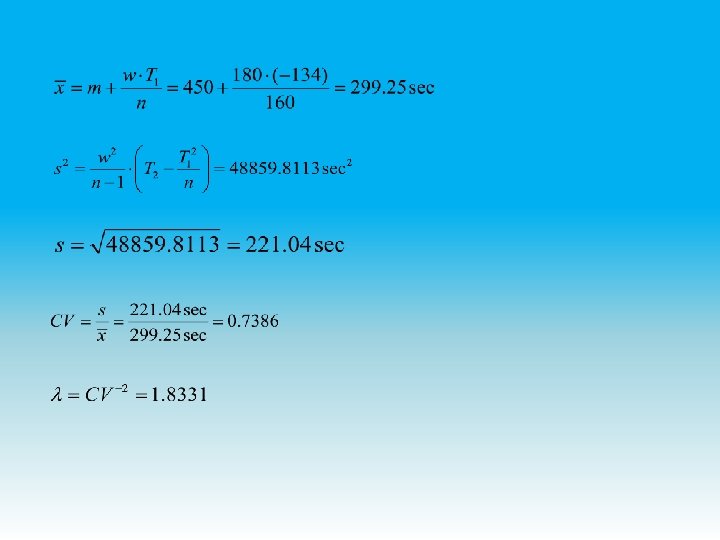
4. We observe a group of insects, sampled randomly, in a laboratory and we write down the surviving individuals at the end of each day. The experiment ends when we see zero insects surviving. It took R=98 days for this (sample range).
 10 28 28 [20, 40) 30")
Classes Class Centers xi ni Ni [0, 20) 10 28 28 [20, 40) 30 23 51 [40, 60) 50 19 70 [60, 80) 70 14 84 [80, 100) 90 12 96 96 Σύνολο
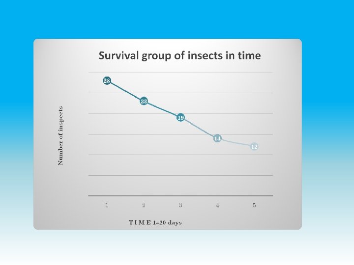

α 0. 2 0. 3 0. 4 0. 5 0. 6 Χ 2 3. 6934 1. 0127 0. 3633 0. 0039 0. 2023 ni Νi n΄i 28 51 70 84 96 when α=0. 5 28. 4 22. 8 18. 3 14. 7 11. 8 96. 0 Classes [0, 20) [20, 40) [40, 60) [60, 80) [80, 100) Total Class centers xi 10 30 50 70 90 28 23 19 14 12 96

α = 0. 5 b = 100 λ = 0. 0110

Type Ι: ν=0. 5695, h=0. 015695, the pdf is given by: Type ΙI: ν=1. 6791, h=0. 015956 , the pdf is given by:

n΄i Type ΙΙ 28. 3 29. 9 24. 6 26. 5 20. 3 21. 0 15. 1 13. 7 7. 7 4. 9 96. 0 Type I: Χ 2 = 2. 6719 Type II: Χ 2 = 3. 7176

CONCLUSION S We can estimate the pdf of a rv Χ from sampling data using only the Coefficient of Variation. In polynomial forms of symmetric, increasing and descending (I, II) distributions, the exponent ν is calculated using only the Coefficient of Variation. Data are better adapted to pdf of descending polynomial form type II compared with type I.

In trigonometric symmetric distributions , the Coefficient of Variation, the parameter λ και the exponent ν are fixed. We can estimate the polynomial pdf of trigonometric distributions from sampling data using the Coefficient of Variation. Polunomial and trigonometric form pdfs assessment methods are equivalent (equally effective).

Data are better adapted to the trigonometric pdf, compared to the polynomial pdf. Data are better adapted in truncated negative exponential distribution rather than in descending ones (I, II).

REFERENCES • A. Muhammad et al. Sk. SP-V Sampling Plan for The Exponentiated Weibull Distribution. Journal of Testing and Evaluation, 42(3): 687– 694, 2013. • D. R. Clark. A Note on the Upper-Truncated Pareto Distribution. Casualty Actuarial Society E-Forum, Winter 2013, 1– 22, 2013. • G. Nanjundan. Estimation of Parameter in a New Truncated Distribution. Open Journal of Statistics, 3(4): 221– 224, 2013. • J. W. Jawitz. Moments of truncated continuous univariate distributions. Advances in Water Resources, 27(3): 269– 281, 2004. • K. Krishnamoorthy. Handbook of Statistical Distribution with Applications. CRC Press, 2006. • L. Sachs. Applied Statistics: A Handbook of Techniques, 2 nd edition. Springer-Verlag Inc. , New York, 1984.

• N. Farmakis. Estimation of Coefficient of Variation: Scaling of Symmetric Continuous Distributions. Statistics in Transition, 6(1): 83– 96, 2003. • N. Farmakis. A Unique Expression for the Size of Samples in Several Sampling Procedures. Statistics in Transition, 7(5): 1031– 1043, 2006. • N. Farmakis. Coefficient of Variation: Connecting Sampling with some Increasing Distribution Models. Proceedings Stochastic Modelling Techniques & Data Analysis International Conference (SMTDA 2010), Chania Crete Greece, 259– 267, 2010. • P. S. Levy, S. Lemeshow. Sampling of Populations: Methods and Applications, 4 th edition. John Wiley & Sons, Inc. , New York, 2008. • T. A. Severini. Elements of Distribution Theory. Cambridge University Press, New York, 2005.

Thank you
- Slides: 49