Poisson distribution Distribution of occurence of rare events

Poisson distribution Distribution of occurence of rare events λ – expected nr. events k – nr. of events Probability of no events (k=0) is e -ℷ ℷ 0=1 Probability of exactly k events is: f(k, ℷ) = (ℷk e-ℷ)/k! 0!=1 COMPULSORY ASSIGNMENT Expected nr. of mutations in corona virus in one year ℷ = 24 Probability of exactly 24 events is: f(24, 24) = (2424 e-24)/24!= 0, 0811 Probability of exactly 0 events is: f(0, 24) = (240 e-24)/0!= 3. 77*10 -11

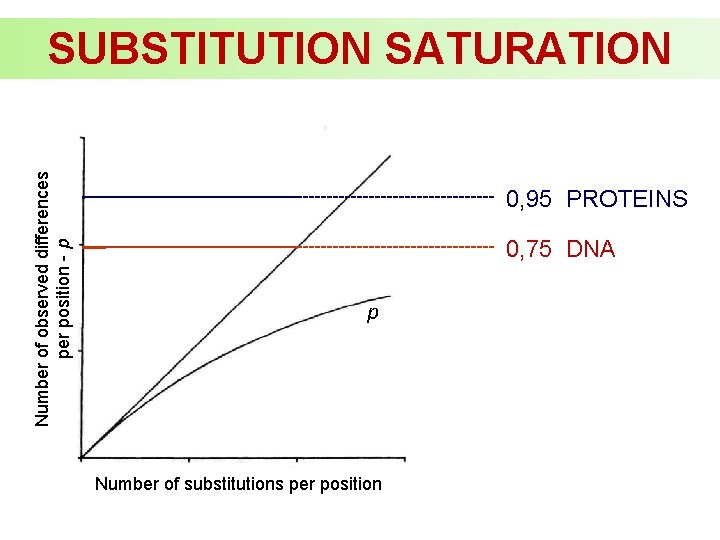
Number of observed differences per position - p SUBSTITUTION SATURATION 0, 95 PROTEINS 0, 75 DNA p Number of substitutions per position

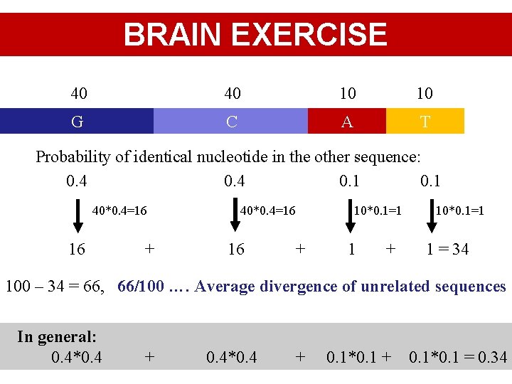
BRAIN EXERCISE 40 40 10 10 G C A T Probability of identical nucleotide in the other sequence: 0. 4 0. 1 40*0. 4=16 16 + 40*0. 4=16 16 10*0. 1=1 + 10*0. 1=1 1 = 34 100 – 34 = 66, 66/100 …. Average divergence of unrelated sequences In general: 0. 4*0. 4 + 0. 1*0. 1 = 0. 34

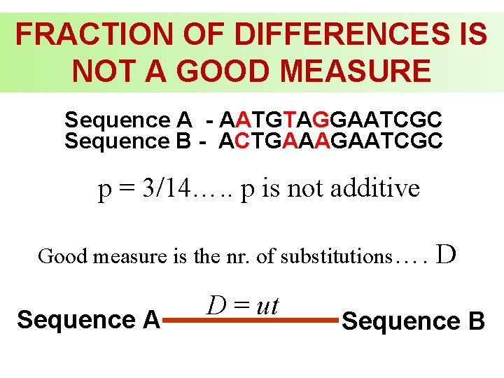
FRACTION OF DIFFERENCES IS NOT A GOOD MEASURE Sequence A - AATGTAGGAATCGC Sequence B - ACTGAAAGAATCGC p = 3/14…. . p is not additive Good measure is the nr. of substitutions…. Sequence A D = ut D Sequence B

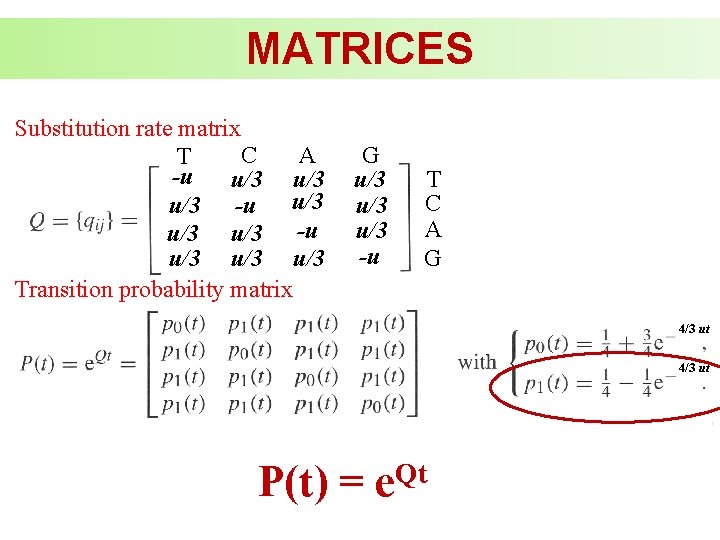
MATRICES Substitution rate matrix C A T -u u/3 u/3 u/3 -u u/3 u/3 Transition probability matrix G u/3 u/3 -u T C A G 4/3 ut P(t) = Qt e

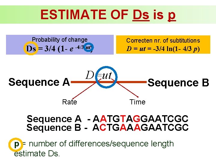
ESTIMATE OF Ds is p Probability of change Correcten nr. of subtitutions Ds = 3/4 (1 - e -4/3 ut) D = ut = -3/4 ln(1 - 4/3 p) Sequence A Rate D=ut Sequence B Time Sequence A - AATGTAGGAATCGC Sequence B - ACTGAAAGAATCGC p = number of differences/sequence length estimate Ds.

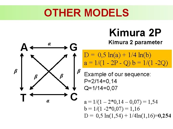
OTHER MODELS Kimura 2 P α A β β β T G α β C Kimura 2 parameter D = 0, 5 ln(a) + 1/4 ln(b) a = 1/(1 - 2 P - Q) b = 1/(1 -2 Q) Example of our sequence: P=2/14=0, 14 Q=1/14=0, 07 a = 1/(1 – 2*0, 14 – 0, 07) = 1, 54 b = 1/(1 -2*0, 07) = 1, 16 D = 0, 5 ln(1, 54) + 1/4 ln(1, 16)=0, 254

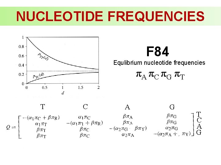
NUCLEOTIDE FREQUENCIES F 84 Equlibrium nucleotide frequencies πA πC πG πT T C A G

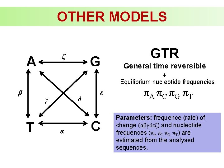
OTHER MODELS ζ A G GTR General time reversible + Equilibrium nucleotide frequencies β δ γ T α ε C πA πC πG πT Parameters: frequence (rate) of change (αβγδεζ) and nucleotide frequences (πA πC πG πT) are estimated from the analysed sequences.

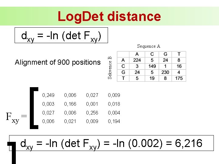
Log. Det distance dxy = -ln (det Fxy) Alignment of 900 positions Fxy = [ Sekvence B Sequence A 0, 249 0, 006 0, 027 0, 009 0, 003 0, 166 0, 001 0, 018 0, 027 0, 006 0, 256 0, 004 0, 006 0, 021 0, 009 0, 194 dxy = -ln (det Fxy) = -ln (0. 002) = 6, 216

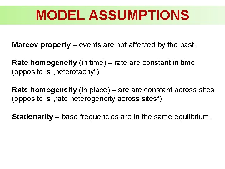
MODEL ASSUMPTIONS Marcov property – events are not affected by the past. Rate homogeneity (in time) – rate are constant in time (opposite is „heterotachy“) Rate homogeneity (in place) – are constant across sites (opposite is „rate heterogeneity across sites“) Stationarity – base frequencies are in the same equlibrium.

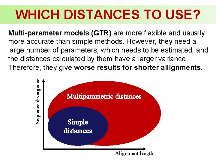
WHICH DISTANCES TO USE? Sequence divergence Multi-parameter models (GTR) are more flexible and usually more accurate than simple methods. However, they need a large number of parameters, which needs to be estimated, and the distances calculated by them have a larger variance. Therefore, they give worse results for shorter allignments. Multiparametric distances Simple distamces Alignment length

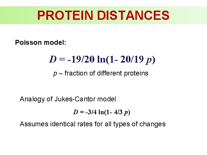
PROTEIN DISTANCES Poisson model: D = -19/20 ln(1 - 20/19 p) p – fraction of different proteins Analogy of Jukes-Cantor model D = -3/4 ln(1 - 4/3 p) Assumes identical rates for all types of changes

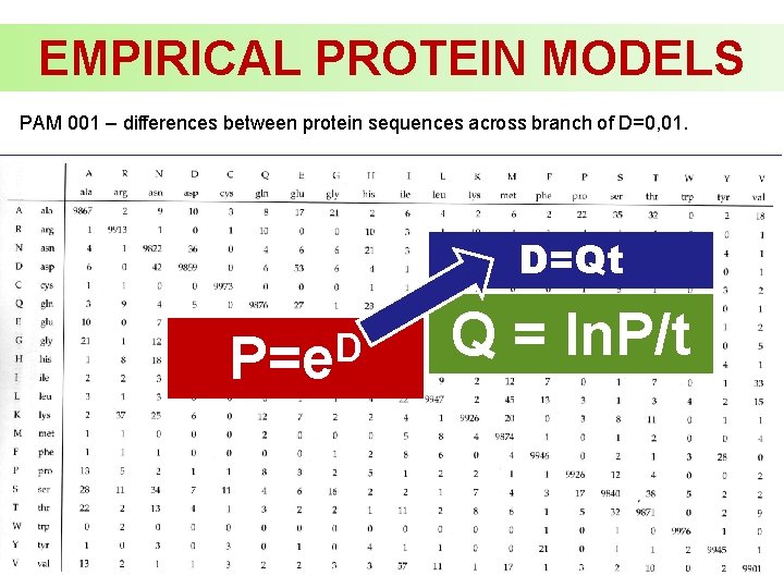
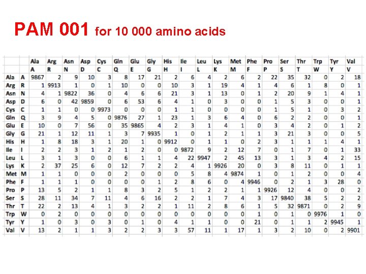
EMPIRICAL PROTEIN MODELS PAM 001 – differences between protein sequences across branch of D=0, 01. D=Qt D P=e Q = ln. P/t

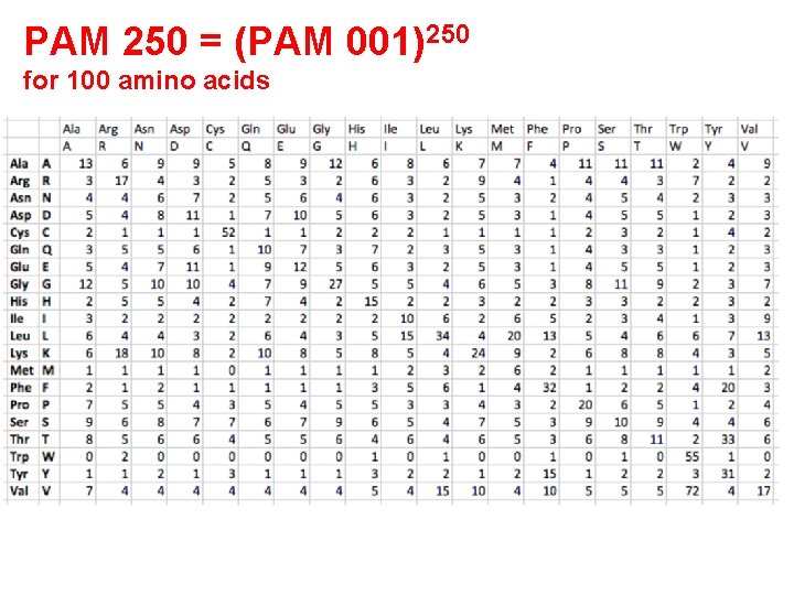
EMPIRICAL PROTEIN MODELS PAM 001 – differences between protein sequences across branch of D=0, 01. Matrix can be recalculated for different D by exponentiation, e. g. D=0, 1 ~ M 10 (PAM 10) D P=e x x. D P =e x D x P =(e )

PAM 001 for 10 000 amino acids

PAM 250 = (PAM 001)250 for 100 amino acids

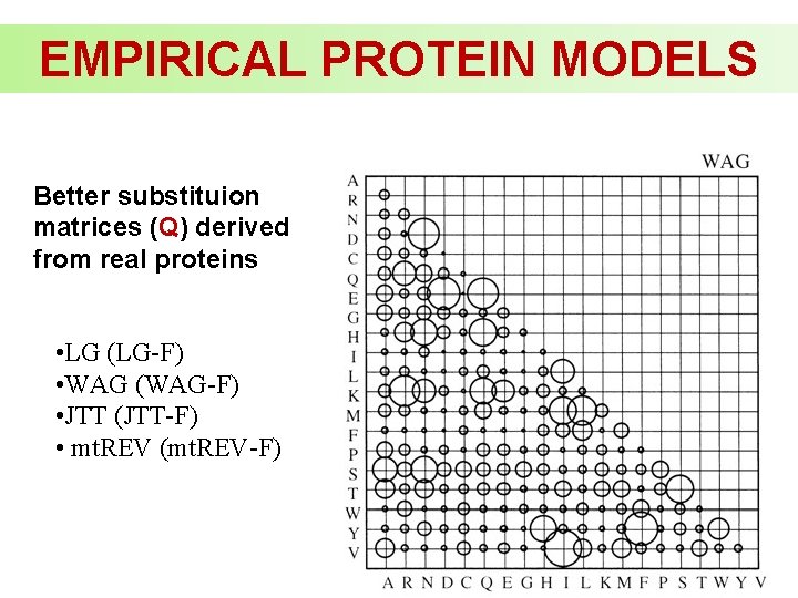
EMPIRICAL PROTEIN MODELS Better substituion matrices (Q) derived from real proteins • LG (LG-F) • WAG (WAG-F) • JTT (JTT-F) • mt. REV (mt. REV-F)

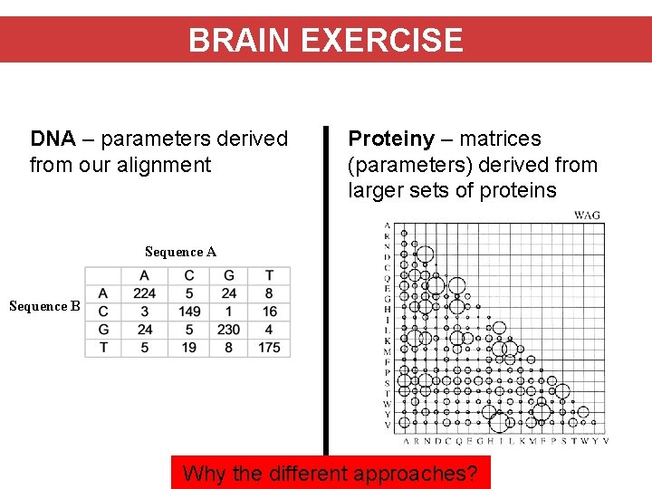
BRAIN EXERCISE DNA – parameters derived from our alignment Proteiny – matrices (parameters) derived from larger sets of proteins Sequence A Sequence B Why the different approaches?

PHYLOGENETIC TREES

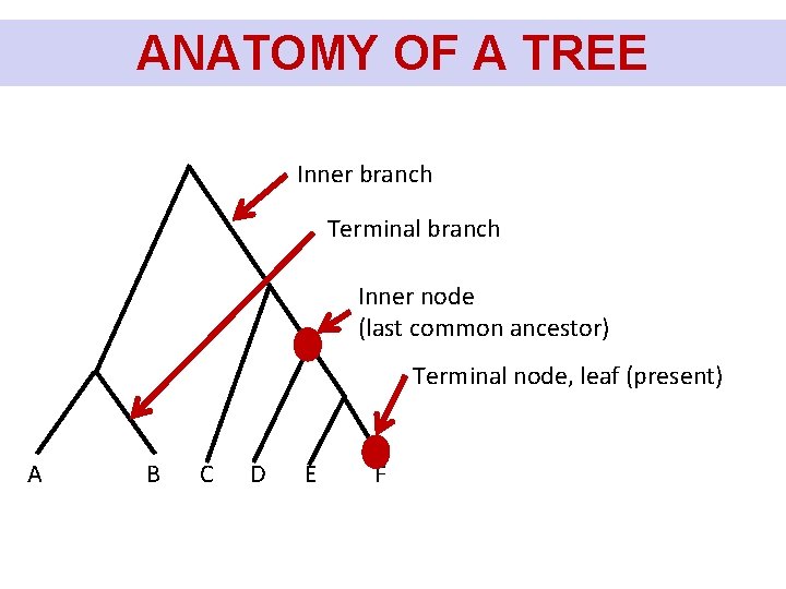
ANATOMY OF A TREE Inner branch Terminal branch Inner node (last common ancestor) Terminal node, leaf (present) A B C D E F

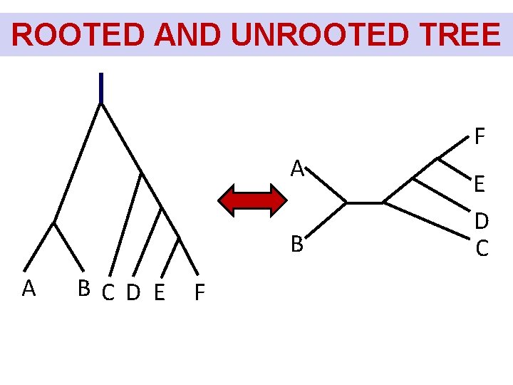
ROOTED AND UNROOTED TREE F A BC D E F E D C

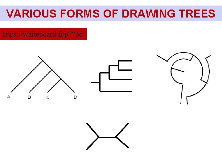
VARIOUS FORMS OF DRAWING TREES https: //whiteboard. fi/p 773 d

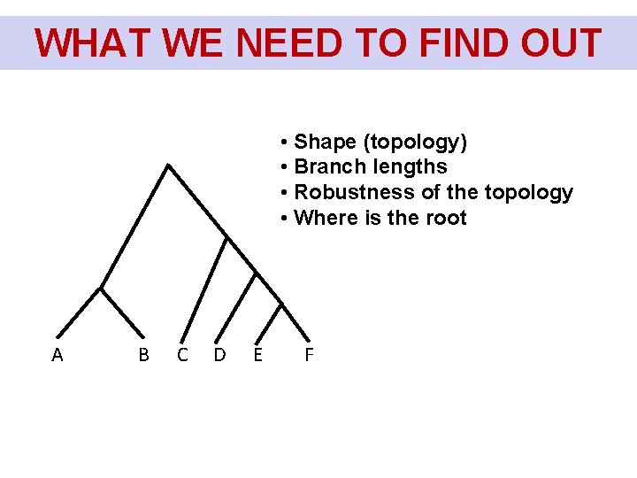
WHAT WE NEED TO FIND OUT Co chceme u stromu zjistit? • Shape (topology) • Branch lengths • Robustness of the topology • Where is the root A B C D E F

HOW TO FIND THE BEST TREE?

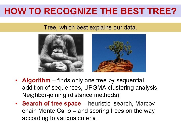
HOW TO RECOGNIZE THE BEST TREE? Tree, which best explains our data. • Algorithm – finds only one tree by sequential addition of sequences, UPGMA clustering analysis, Neighbor-joining (distance methods). • Search of tree space – heuristic search, Marcov chain Monte Carlo – and scoring trees on the way according to various criteria.

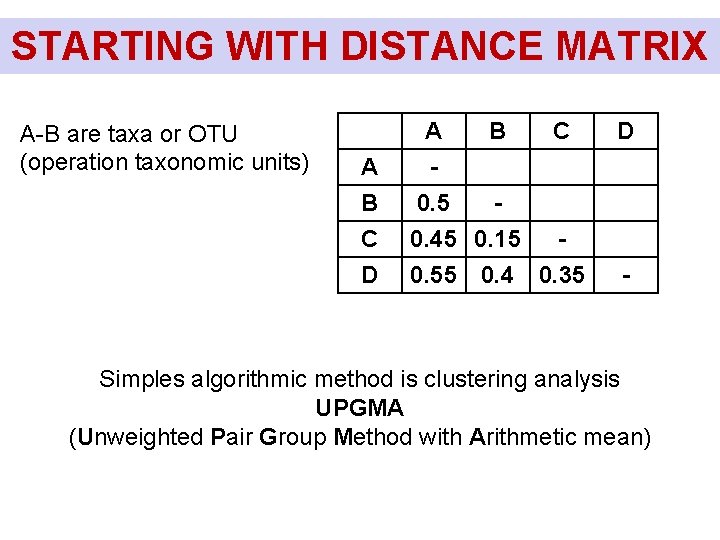
STARTING WITH DISTANCE MATRIX A-B are taxa or OTU (operation taxonomic units) A B C A B 0. 5 0. 45 0. 15 D 0. 55 0. 4 C D 0. 35 - Simples algorithmic method is clustering analysis UPGMA (Unweighted Pair Group Method with Arithmetic mean)

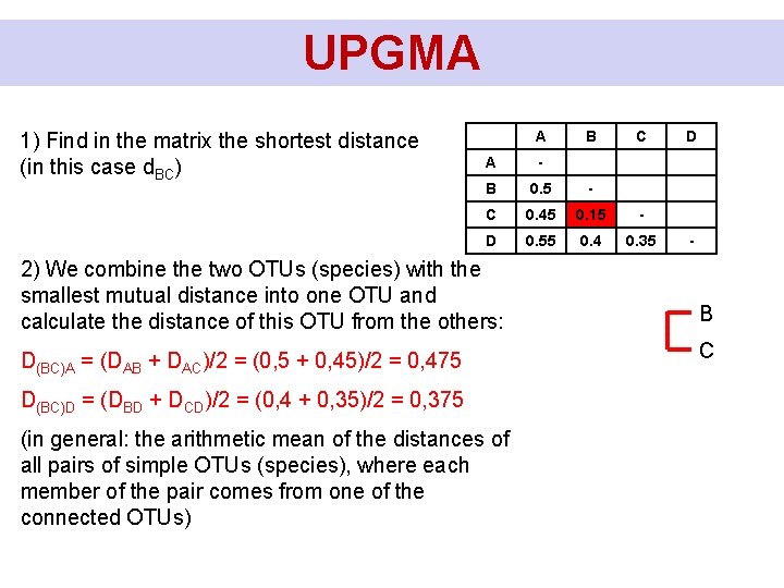
UPGMA 1) Find in the matrix the shortest distance (in this case d. BC) A B C A - B 0. 5 - C 0. 45 0. 15 - D 0. 55 0. 4 0. 35 2) We combine the two OTUs (species) with the smallest mutual distance into one OTU and calculate the distance of this OTU from the others: D(BC)A = (DAB + DAC)/2 = (0, 5 + 0, 45)/2 = 0, 475 D(BC)D = (DBD + DCD)/2 = (0, 4 + 0, 35)/2 = 0, 375 (in general: the arithmetic mean of the distances of all pairs of simple OTUs (species), where each member of the pair comes from one of the connected OTUs) D - B C

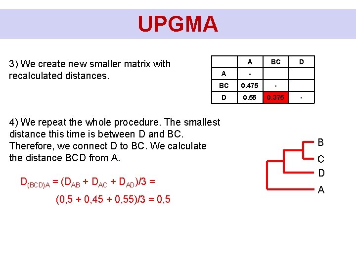
UPGMA A 3) We create new smaller matrix with recalculated distances. A - BC 0. 475 - D 0. 55 0. 375 4) We repeat the whole procedure. The smallest distance this time is between D and BC. Therefore, we connect D to BC. We calculate the distance BCD from A. D(BCD)A = (DAB + DAC + DAD)/3 = (0, 5 + 0, 45 + 0, 55)/3 = 0, 5 BC D - B C D A

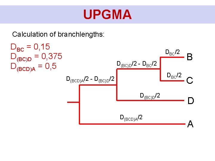
UPGMA Calculation of branchlengths: DBC = 0, 15 D(BC)D = 0, 375 D(BCD)A = 0, 5 DBC/2 D(BC)D/2 - DBC/2 D(BCD)A/2 - D(BC)D/2 D(BCD)A/2 B C D A

UPGMA Calculation of branchlengths: DBC = 0, 15 D(BC)D = 0, 375 D(BCD)A = 0, 5 0, 075 D(BC)D/2 - DBC/2 0, 075 D(BCD)A/2 - D(BC)D/2 D(BCD)A/2 B C D A

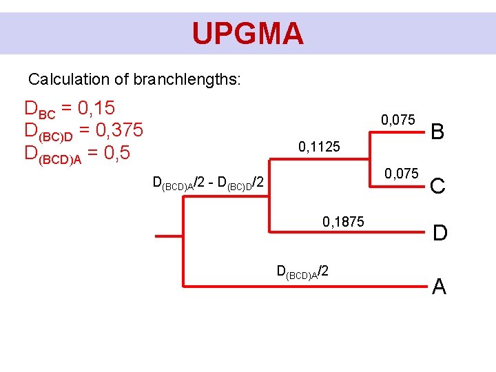
UPGMA Calculation of branchlengths: DBC = 0, 15 D(BC)D = 0, 375 D(BCD)A = 0, 5 0, 075 0, 1125 0, 075 D(BCD)A/2 - D(BC)D/2 0, 1875 D(BCD)A/2 B C D A

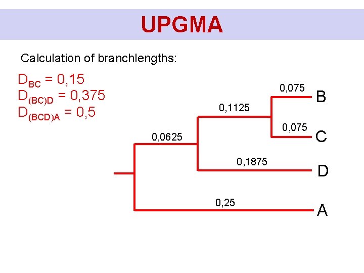
UPGMA Calculation of branchlengths: DBC = 0, 15 D(BC)D = 0, 375 D(BCD)A = 0, 5 0, 075 0, 1125 0, 075 0, 0625 0, 1875 0, 25 B C D A

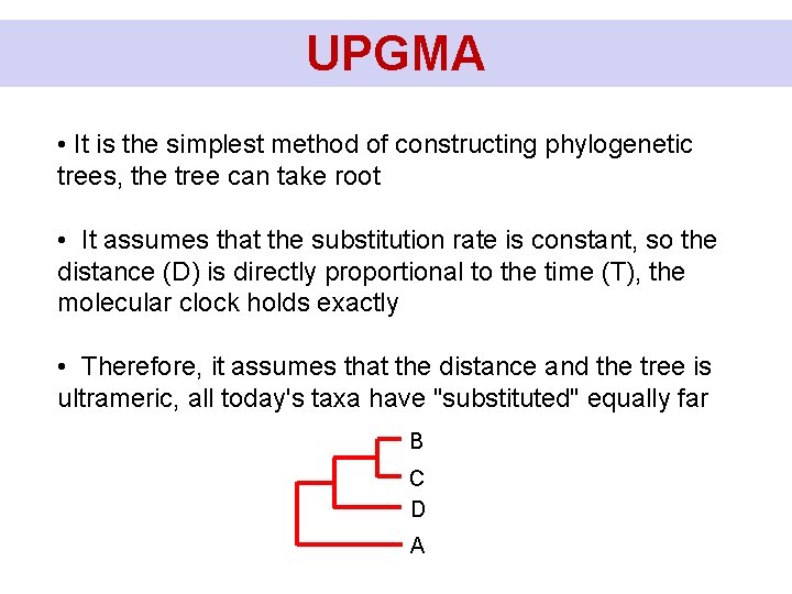
UPGMA • It is the simplest method of constructing phylogenetic trees, the tree can take root • It assumes that the substitution rate is constant, so the distance (D) is directly proportional to the time (T), the molecular clock holds exactly • Therefore, it assumes that the distance and the tree is ultrameric, all today's taxa have "substituted" equally far B C D A

UPGMA • However, these assumptions are almost always violated • If the assumptions are violated significantly, the method will simply confuse and give a wrong tree • It tends to move more divergent sequences closer to the root of the tree - the artifact of attracting long branches (LBA) • LBA is one of the biggest pitfalls of molecular phylogenetics

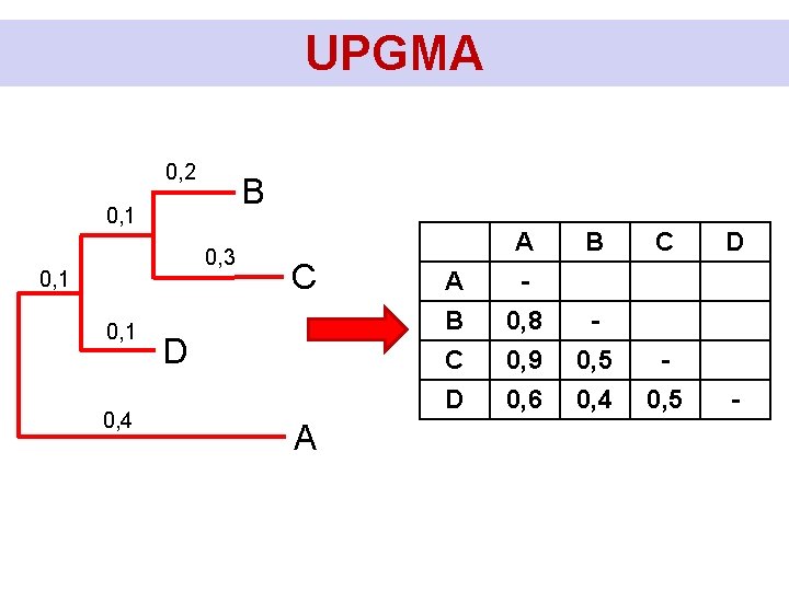
UPGMA 0, 2 B 0, 1 0, 3 0, 1 0, 4 C D A B C A 0, 8 0, 9 0, 5 - D 0, 6 0, 4 0, 5 D -

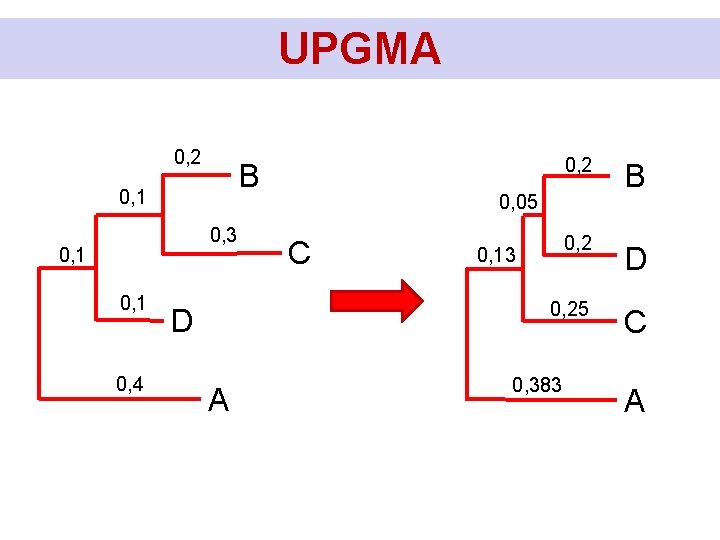
UPGMA 0, 2 B 0, 1 0, 3 0, 1 0, 4 D A 0, 2 B 0, 2 D 0, 25 C 0, 05 C 0, 13 0, 383 A

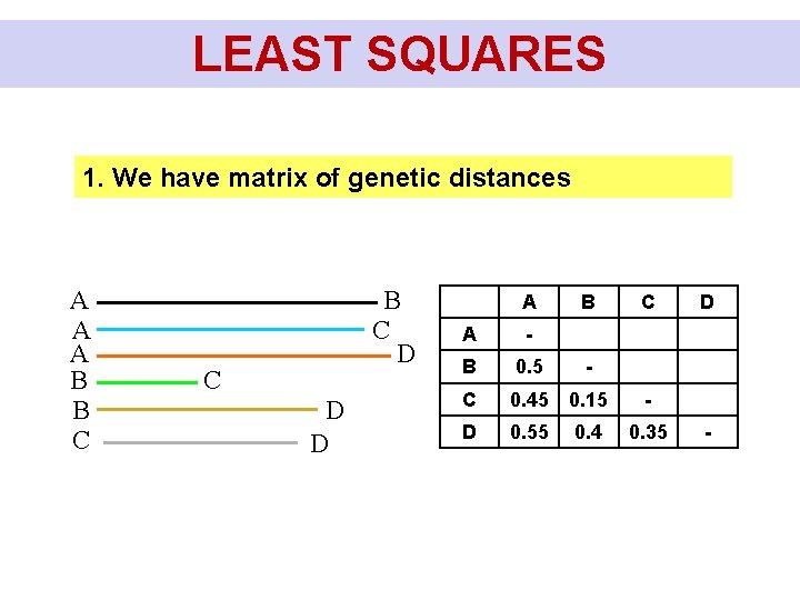
LEAST SQUARES 1. We have matrix of genetic distances A A A B B C D C D D A B C A - B 0. 5 - C 0. 45 0. 15 - D 0. 55 0. 4 0. 35 D -

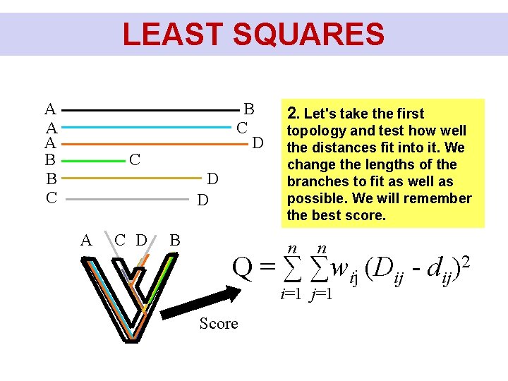
LEAST SQUARES A A A B B C D C D D A C D B 2. Let's take the first topology and test how well the distances fit into it. We change the lengths of the branches to fit as well as possible. We will remember the best score. n n Q = ∑ ∑wij (Dij - dij)2 i=1 j=1 Score

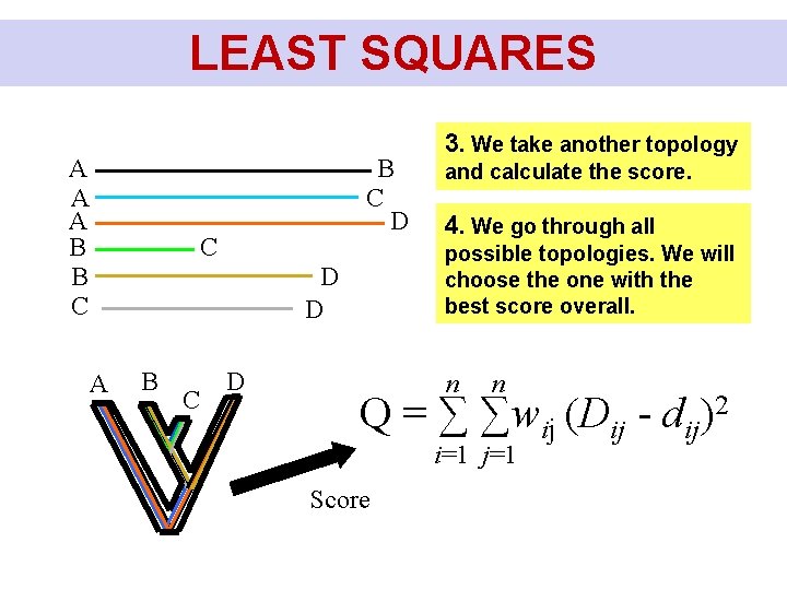
LEAST SQUARES A A A B B C D C B C D and calculate the score. 4. We go through all possible topologies. We will choose the one with the best score overall. D D A 3. We take another topology n n Q = ∑ ∑wij (Dij - dij)2 i=1 j=1 Score

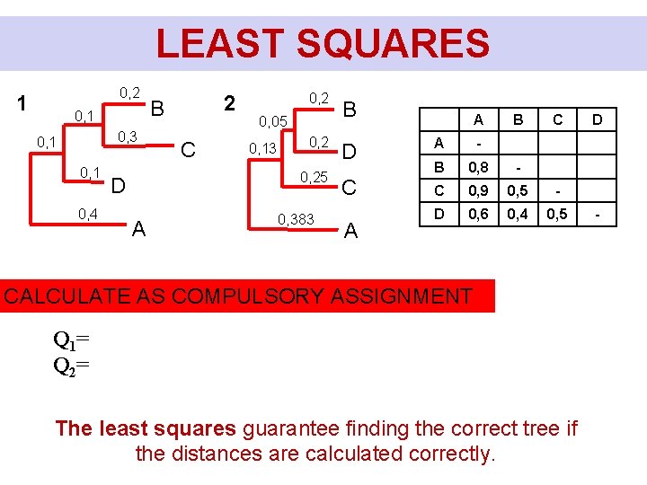
LEAST SQUARES 0, 2 1 0, 3 0, 1 0, 4 2 B C 0, 2 0, 05 0, 13 0, 25 D A 0, 383 B D C A A B C A - B 0, 8 - C 0, 9 0, 5 - D 0, 6 0, 4 0, 5 CALCULATE AS COMPULSORY ASSIGNMENT Q 1= Q 2= The least squares guarantee finding the correct tree if the distances are calculated correctly. D -