PNNL Network modeling is dead long live network

PNNL Network modeling is dead, long live network modeling Anthony Bonato Ryerson University

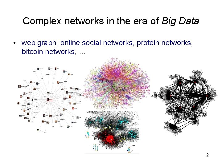
Complex networks in the era of Big Data • web graph, online social networks, protein networks, bitcoin networks, … 2

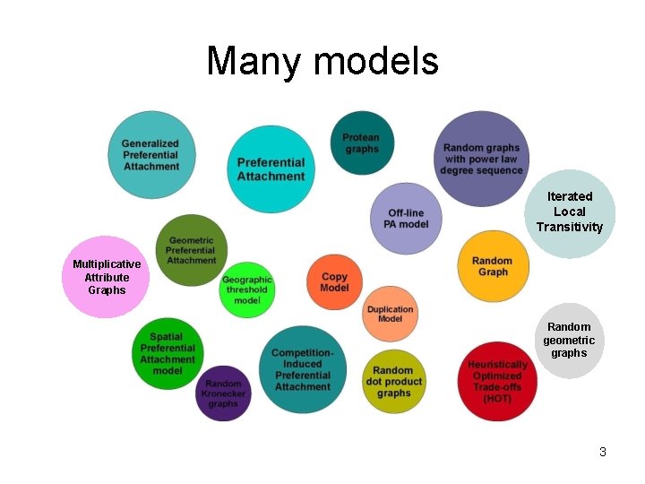
Many models Iterated Local Transitivity Multiplicative Attribute Graphs Random geometric graphs 3

Questions and Cases 1. What do network models tell us about reality? a. dimensions of social space b. character networks 2. What are the limits of models? a. Cops and Robbers b. Zombies and Survivors 4

Case 1 a: Dimensions of social networks 5

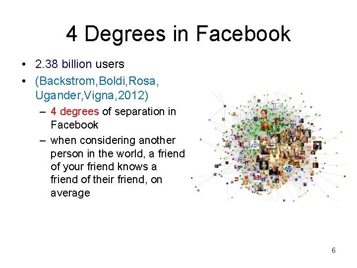
4 Degrees in Facebook • 2. 38 billion users • (Backstrom, Boldi, Rosa, Ugander, Vigna, 2012) – 4 degrees of separation in Facebook – when considering another person in the world, a friend of your friend knows a friend of their friend, on average 6

Social distance • 4 degrees of separation does not reflect our true social distance D. Liben-Nowell, J. Kleinberg, Tracing information flow on a global scale using Internet chain-letter data PNAS 105 (2008) 4633 -4638. 7

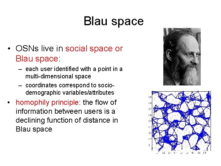
Blau space • OSNs live in social space or Blau space: – each user identified with a point in a multi-dimensional space – coordinates correspond to sociodemographic variables/attributes • homophily principle: the flow of information between users is a declining function of distance in Blau space 8

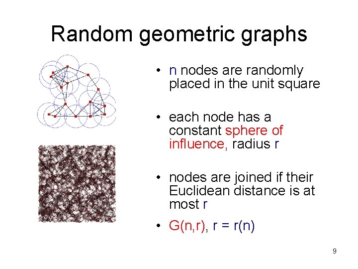
Random geometric graphs • n nodes are randomly placed in the unit square • each node has a constant sphere of influence, radius r • nodes are joined if their Euclidean distance is at most r • G(n, r), r = r(n) 9

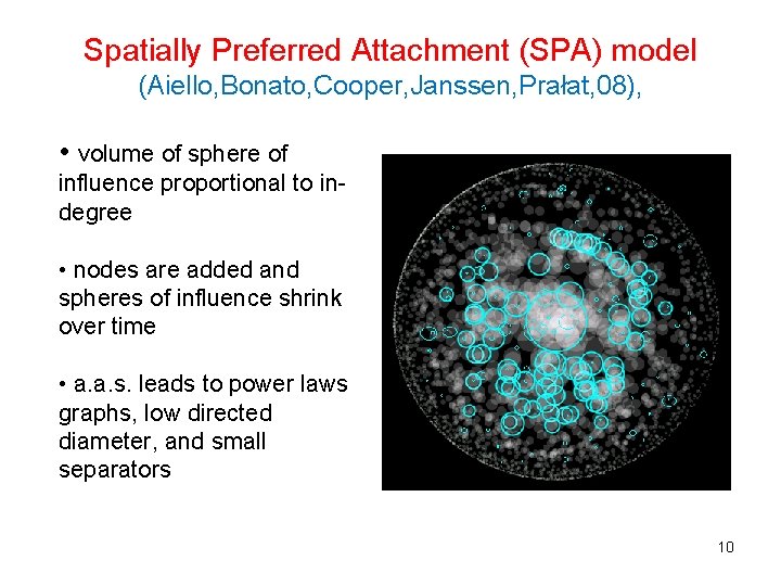
Spatially Preferred Attachment (SPA) model (Aiello, Bonato, Cooper, Janssen, Prałat, 08), • volume of sphere of influence proportional to indegree • nodes are added and spheres of influence shrink over time • a. a. s. leads to power laws graphs, low directed diameter, and small separators 10

Ranking models (Fortunato, Flammini, Menczer, 06), (Łuczak, Prałat, 06), (Janssen, Prałat, 09) • parameter: α in (0, 1) • each node is ranked 1, 2, …, n by some function r – 1 is best, n is worst • at each time-step, one new node is born, one randomly node chosen dies (and ranking is updated) • link probability r-α • many ranking schemes a. a. s. lead to power law graphs: random initial ranking, degree, age, etc. 11

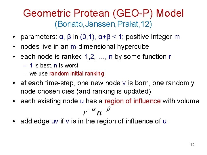
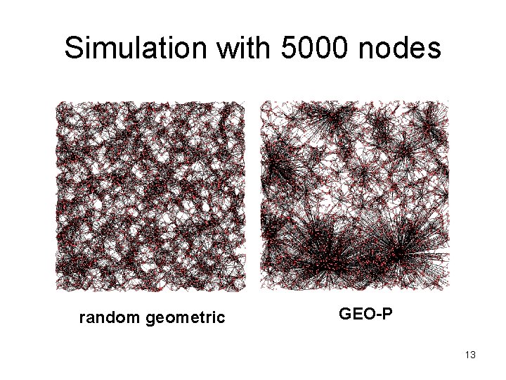
Geometric Protean (GEO-P) Model (Bonato, Janssen, Prałat, 12) • parameters: α, β in (0, 1), α+β < 1; positive integer m • nodes live in an m-dimensional hypercube • each node is ranked 1, 2, …, n by some function r – 1 is best, n is worst – we use random initial ranking • at each time-step, one new node v is born, one randomly node chosen dies (and ranking is updated) • each existing node u has a region of influence with volume • add edge uv if v is in the region of influence of u 12

Simulation with 5000 nodes random geometric GEO-P 13

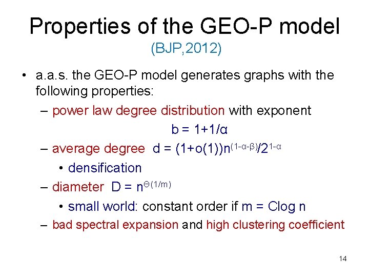
Properties of the GEO-P model (BJP, 2012) • a. a. s. the GEO-P model generates graphs with the following properties: – power law degree distribution with exponent b = 1+1/α – average degree d = (1+o(1))n(1 -α-β)/21 -α • densification – diameter D = nΘ(1/m) • small world: constant order if m = Clog n – bad spectral expansion and high clustering coefficient 14

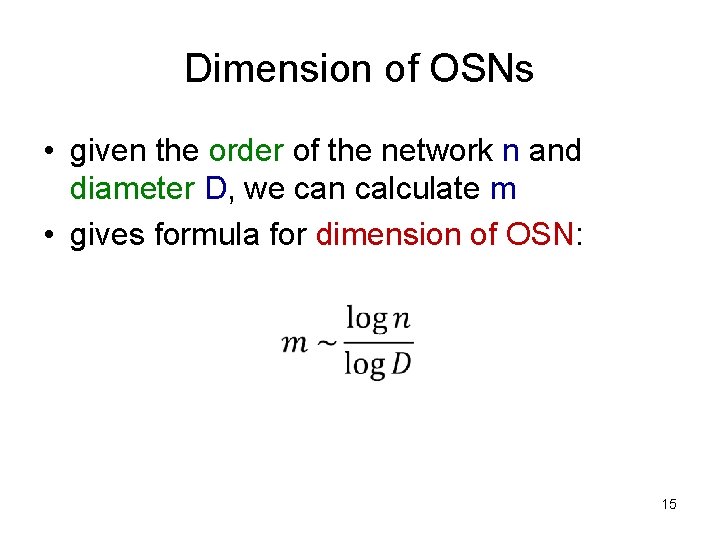
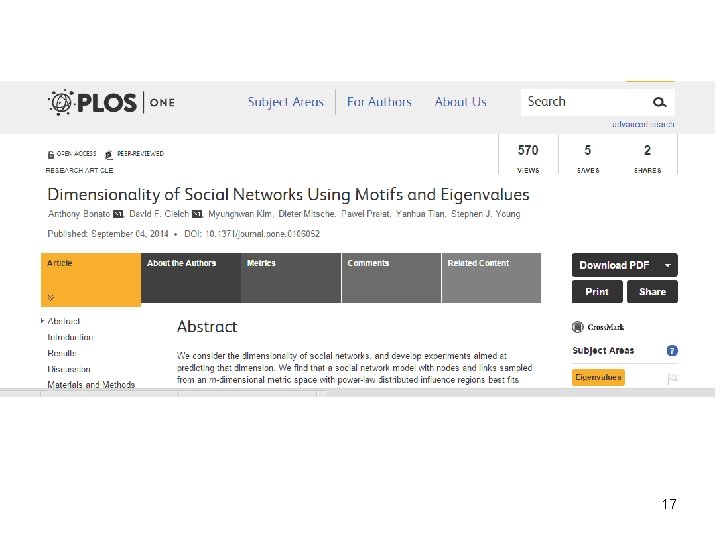
Dimension of OSNs • given the order of the network n and diameter D, we can calculate m • gives formula for dimension of OSN: 15

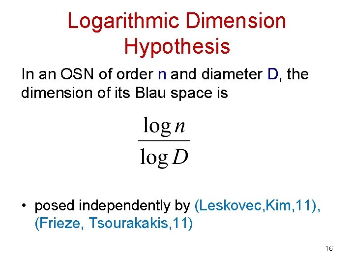
Logarithmic Dimension Hypothesis In an OSN of order n and diameter D, the dimension of its Blau space is • posed independently by (Leskovec, Kim, 11), (Frieze, Tsourakakis, 11) 16

17

Model selection in complex networks • (Middendorf, Ziv, Wiggins, 05) – used ADTs and motifs for model selection in protein networks – predicted duplication/mutation model • (Memišević, Milenković, Pržulj, 10) – model selection predicting random geometric graphs as best fit for protein networks • (Janssen, Hurshman, Kalyaniwalla, 12) – ADT with motif classifiers predict PA and SPA models best fit Facebook 100 graphs 18

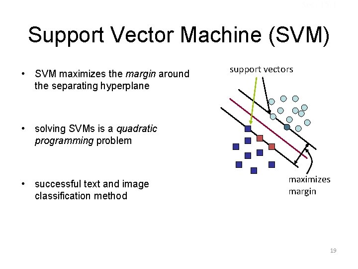
Sec. 15. 1 Support Vector Machine (SVM) • SVM maximizes the margin around the separating hyperplane support vectors • solving SVMs is a quadratic programming problem • successful text and image classification method maximizes margin 19

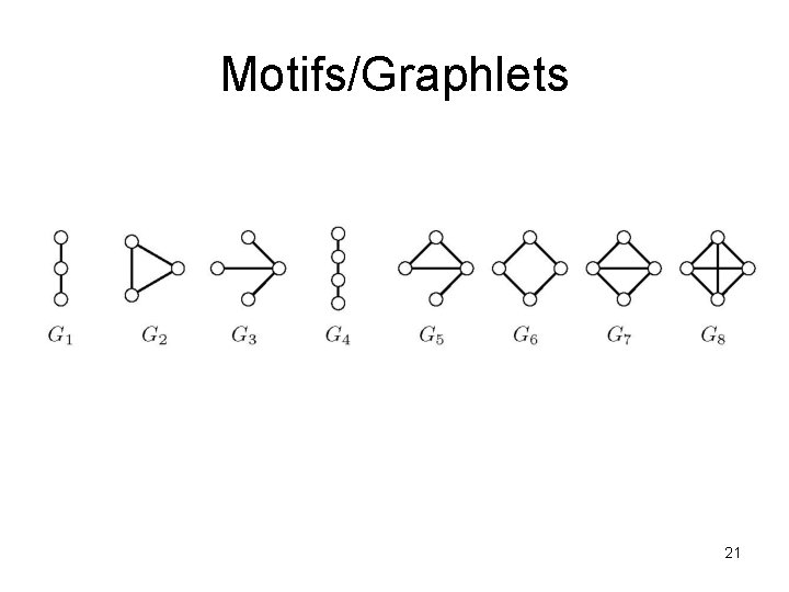
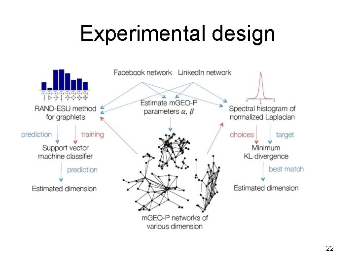
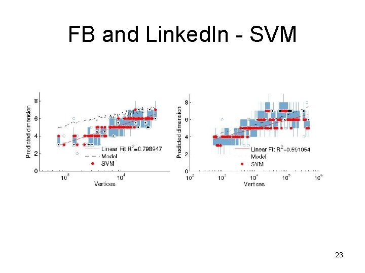
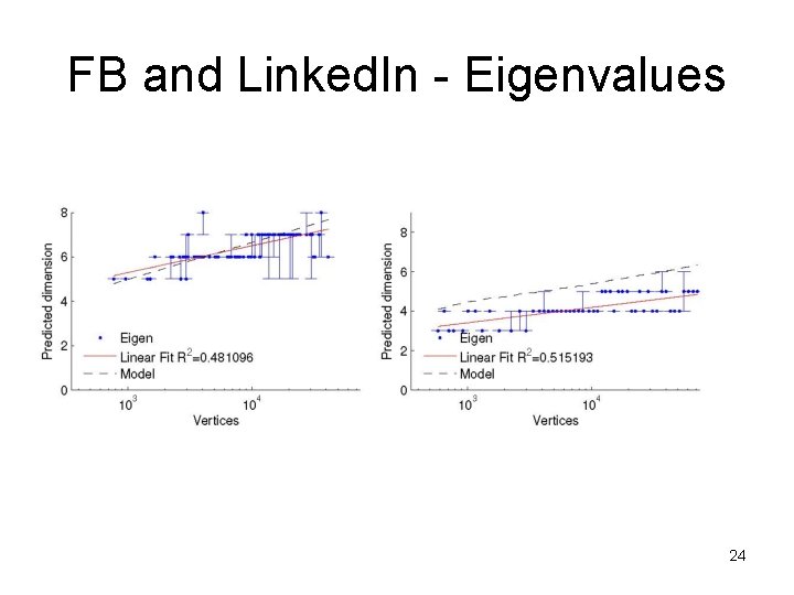
Validating the LDH • we tested the dimensionality of large-scale samples from real OSN data – FB 100 and Linked. In (sampled over time) • Idea: use machine learning (SVM) to predict dimensions – features: small subgraph counts (3 - and 4 -vertex subgraphs) – compared sampled data vs simulations of MGEO-P with dimensions 1 through 12 20

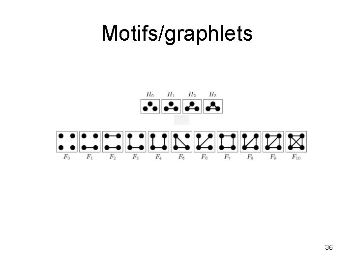
Motifs/Graphlets 21

Experimental design 22

FB and Linked. In - SVM 23

FB and Linked. In - Eigenvalues 24

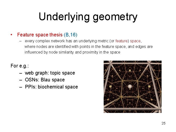
Underlying geometry • Feature space thesis (B, 16) – every complex network has an underlying metric (or feature) space, where nodes are identified with points in the feature space, and edges are influenced by node similarity and proximity in the space For e. g. : – web graph: topic space – OSNs: Blau space – PPIs: biochemical space 25

Case 1 b: Character Networks 26

Character networks • cultural work: – fictional works such novels or short stories, movies, biographies, historical works, religious texts • character networks: – nodes: characters or persona in a cultural work – edges: co-occurrence • edges may be weighted 27

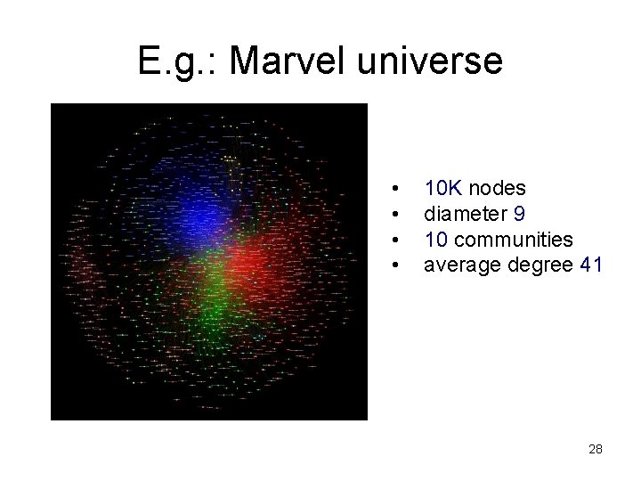
E. g. : Marvel universe • • 10 K nodes diameter 9 10 communities average degree 41 28

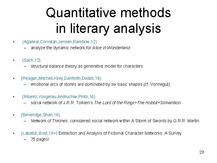
Quantitative methods in literary analysis • (Agarwal, Corvalan, Jensen, Rambow, 12) – analyze the dynamic network for Alice in Wonderland • (Sack, 12) – structural balance theory as generative model for characters • (Reagan, Mitchell, Kiley, Danforth, Dodds, 16) – emotional arcs of stories are dominated by six basic shapes (cf. Vonnegut) • (Ribeiro, Vosgerau, Andruchiw, Pinto, 16) – social network of J. R. R. Tolkien’s The Lord of the Rings+The Hobbit+Silmarillion • (Beveridge, Shan, 16) – Network of Thrones: considered social network within A Storm of Swords by G. R. R. Martin • (Labatut, Bost, 19+) Extraction and Analysis of Fictional Character Networks: A Survey – 75 pages! 29

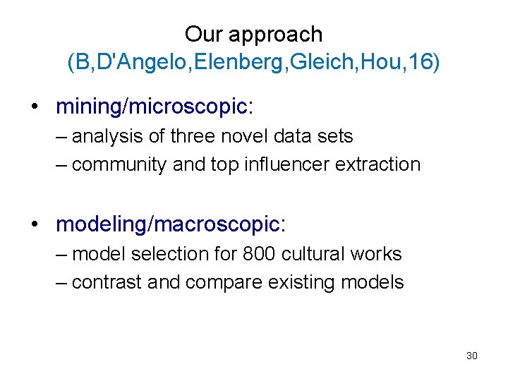
Our approach (B, D'Angelo, Elenberg, Gleich, Hou, 16) • mining/microscopic: – analysis of three novel data sets – community and top influencer extraction • modeling/macroscopic: – model selection for 800 cultural works – contrast and compare existing models 30

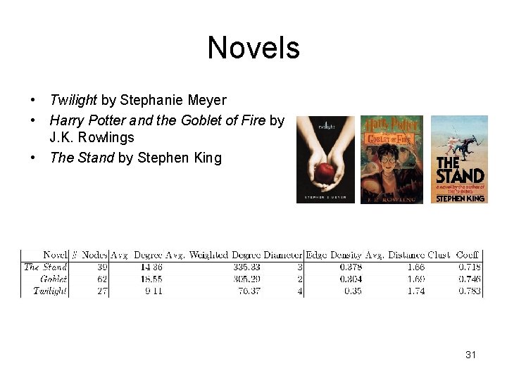
Novels • Twilight by Stephanie Meyer • Harry Potter and the Goblet of Fire by J. K. Rowlings • The Stand by Stephen King 31

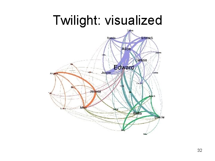
Twilight: visualized 32

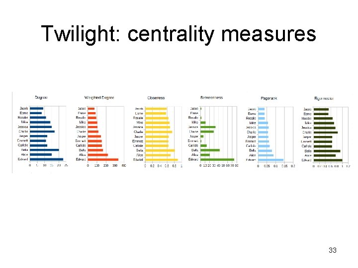
Twilight: centrality measures 33

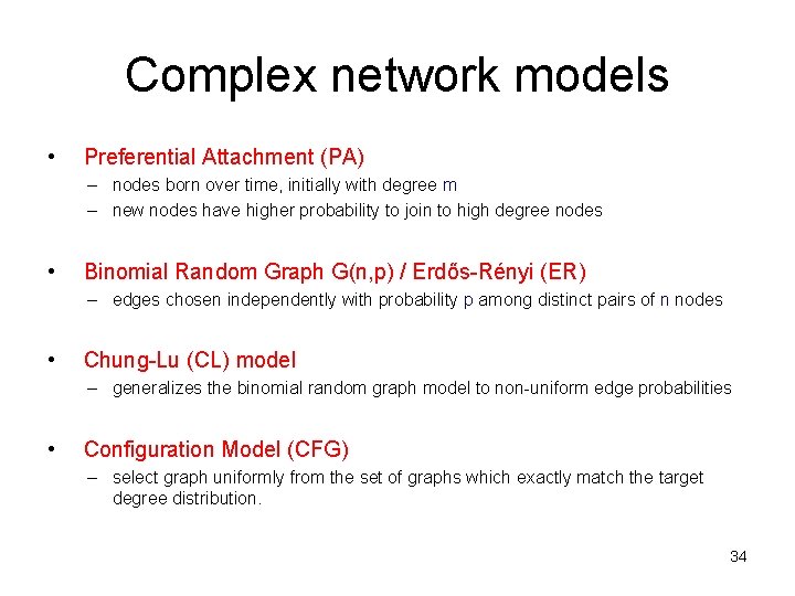
Complex network models • Preferential Attachment (PA) – nodes born over time, initially with degree m – new nodes have higher probability to join to high degree nodes • Binomial Random Graph G(n, p) / Erdős-Rényi (ER) – edges chosen independently with probability p among distinct pairs of n nodes • Chung-Lu (CL) model – generalizes the binomial random graph model to non-uniform edge probabilities • Configuration Model (CFG) – select graph uniformly from the set of graphs which exactly match the target degree distribution. 34

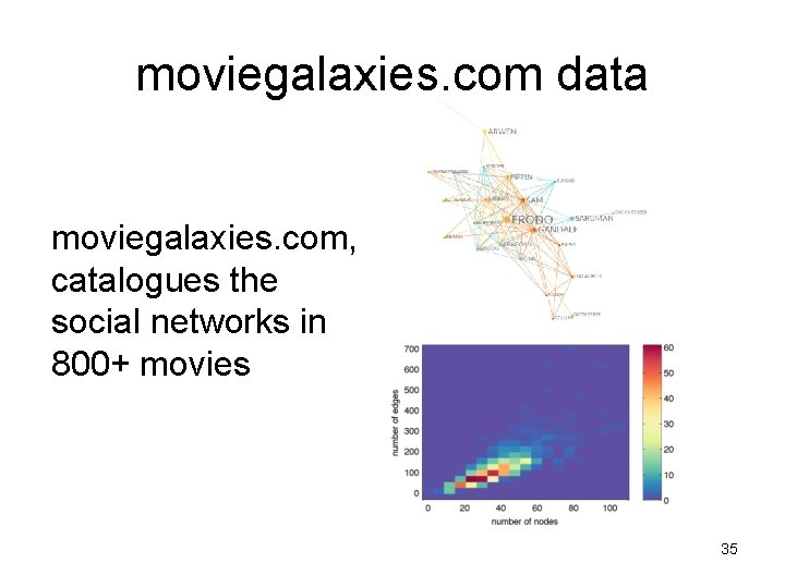
moviegalaxies. com data moviegalaxies. com, catalogues the social networks in 800+ movies 35

Motifs/graphlets 36

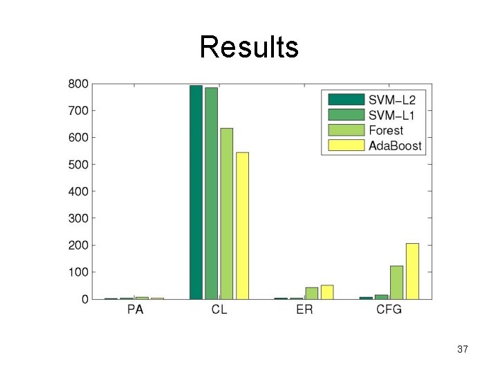
Results 37

Conclusions • CL best fitting model for 800+ samples – tested with four ML algorithms – tested also via comparisons with eigenvalue spectrum • why CL? – author may intuit a hierarchy of character influence (via degrees), then randomly generate the social ties – eg Rowlings may have decided the main triad was Harry, Hermione and Ron, and then gradually added lesser characters revolving around this triad 38

Case 2 a: Cops and Robbers 39

40

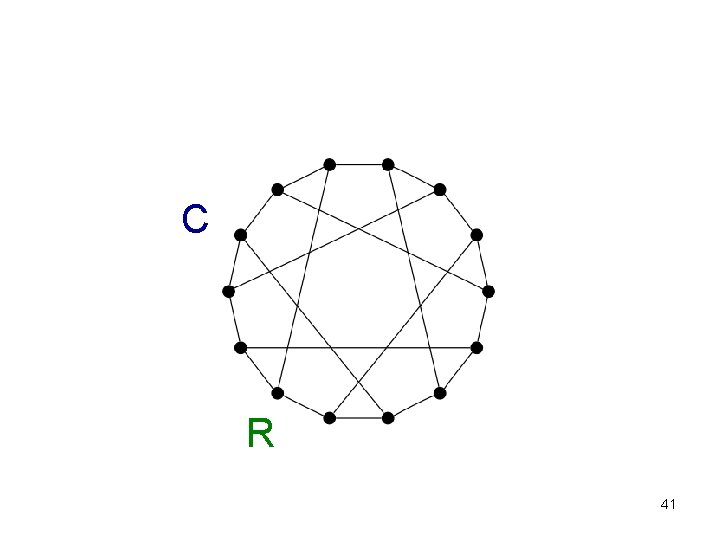
C R 41

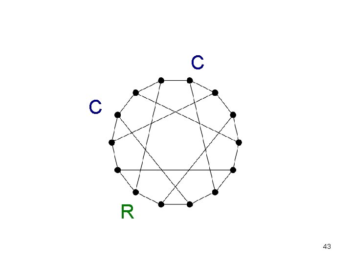
C R 42

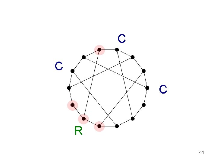
C C R 43

C C C R 44

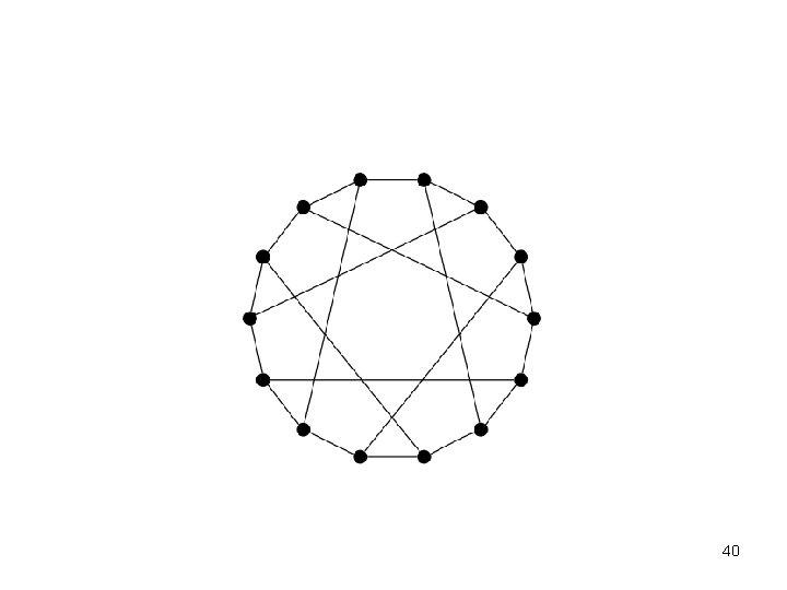
A model for pursuit-evasion: Cops and Robbers • two players Cops C and robber R play at alternate time-steps (cops first) with perfect information • players move to vertices along edges; may move to neighbors or pass • cops try to capture (i. e. land on) the robber, while robber tries to evade capture 45

Cops and Robbers • minimum number of cops needed to capture the robber is the cop number c(G) – well-defined as c(G) ≤ |V(G)| 46

47

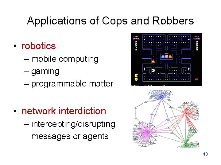
Applications of Cops and Robbers • robotics – mobile computing – gaming – programmable matter • network interdiction – intercepting/disrupting messages or agents 48

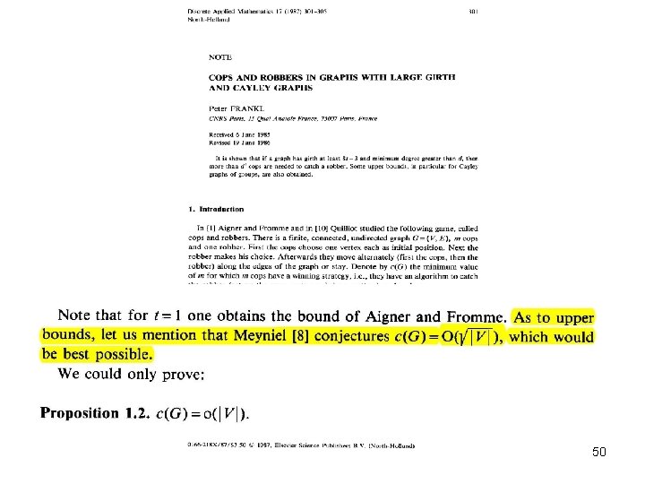
Limits of our understanding of cop number • if G is disconnected, then we can have c(G) = n • define c(n) to be the maximum value of c(G) for a connected G of order n Meyniel’s Conjecture: c(n) = O(n 1/2). 49

50

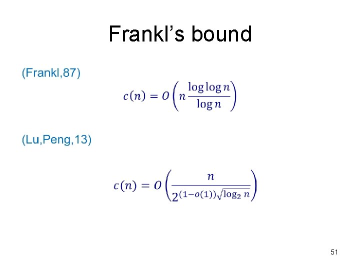
Frankl’s bound • 51

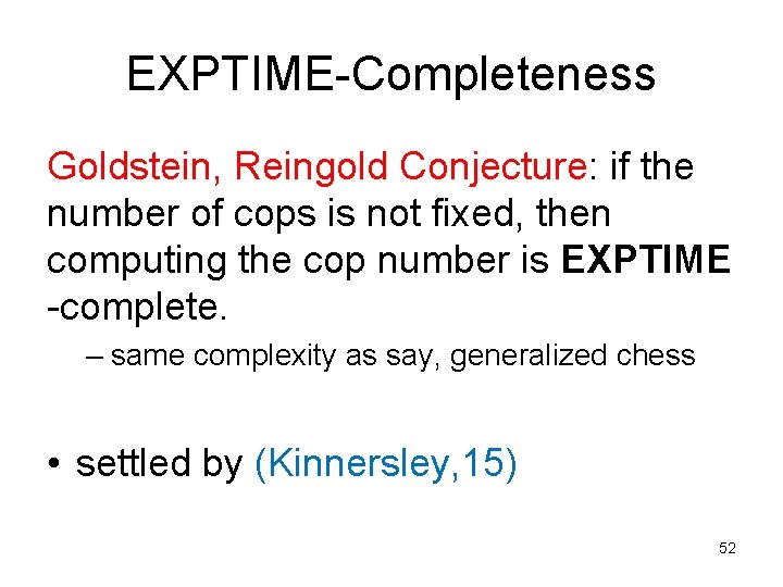
EXPTIME-Completeness Goldstein, Reingold Conjecture: if the number of cops is not fixed, then computing the cop number is EXPTIME -complete. – same complexity as say, generalized chess • settled by (Kinnersley, 15) 52

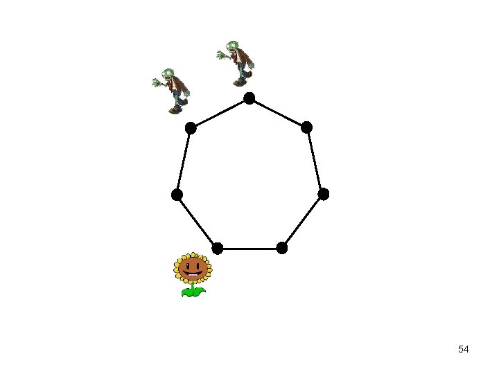
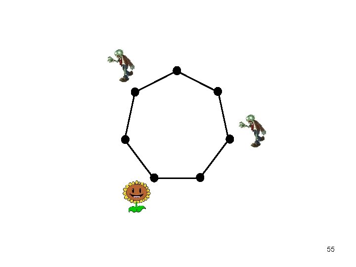
Case 2 a: Zombies and Survivors 53

54

55

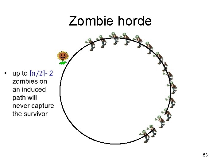
Zombie horde 56

Zombies and Survivors • set of zombies, one survivor • players move at alternate ticks of the clock, from vertex to vertex along edges • zombies choose their initial locations u. a. r. • at each step the zombies move along a shortest path connected to the survivor – if more than one such path, then they choose one u. a. r. • zombies win if one or more can eat the survivor – land on the survivor’s vertex • otherwise, survivor wins • NB: zombies have no strategy! 57

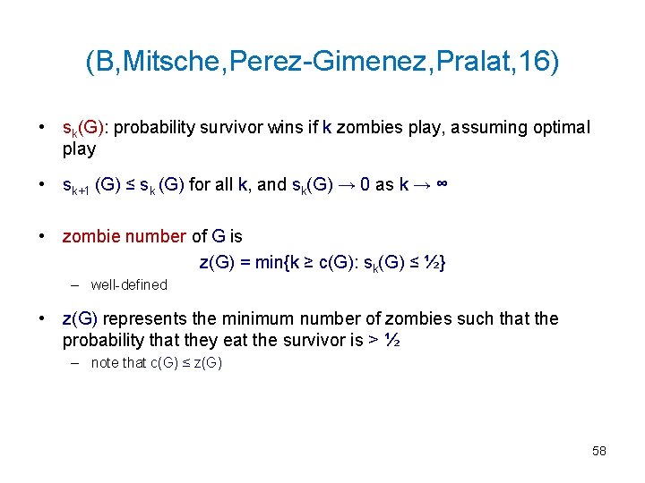
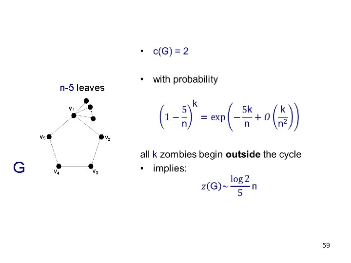
(B, Mitsche, Perez-Gimenez, Pralat, 16) • sk(G): probability survivor wins if k zombies play, assuming optimal play • sk+1 (G) ≤ sk (G) for all k, and sk(G) → 0 as k → ∞ • zombie number of G is z(G) = min{k ≥ c(G): sk(G) ≤ ½} – well-defined • z(G) represents the minimum number of zombies such that the probability that they eat the survivor is > ½ – note that c(G) ≤ z(G) 58

n-5 leaves G 59

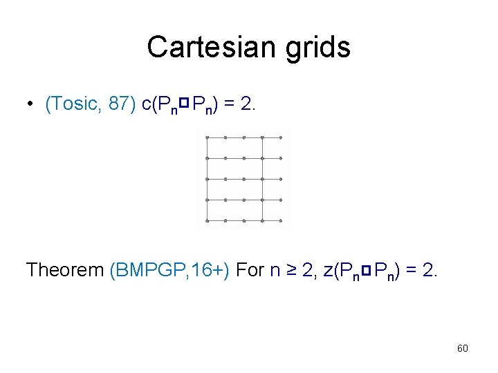
Cartesian grids • (Tosic, 87) c(Pn Pn) = 2. Theorem (BMPGP, 16+) For n ≥ 2, z(Pn Pn) = 2. 60

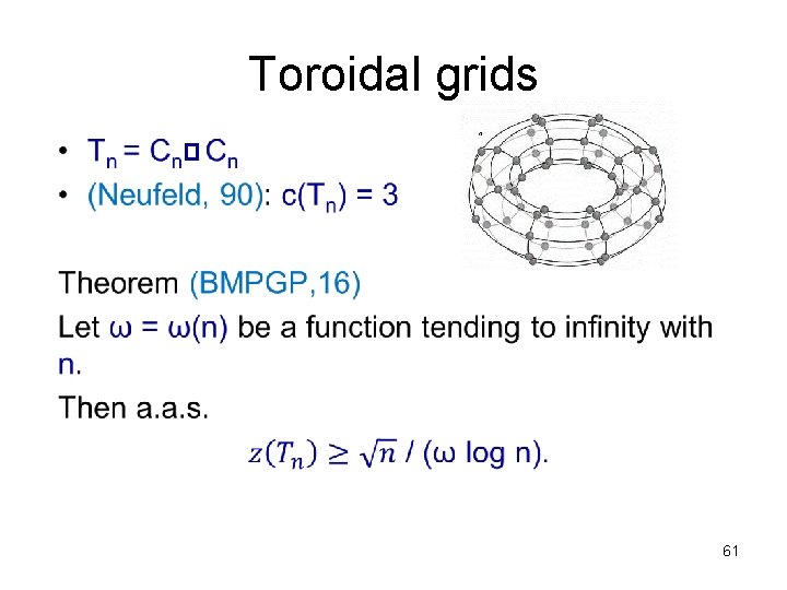
Toroidal grids • 61

Toroidal grids, continued • despite the lower bound, no known subquadratic bound is known for the zombie number of toroidal graphs! • Open Problem: determine the zombie number of the toroidal grid. 62

Contact • Web: http: //www. math. ryerson. ca/~abonato/ • Blog: https: //anthonybonato. com/ • @Anthony_Bonato • https: //www. facebook. com/anthony. bonato. 5