PLT 328 ROBOTICS CONTROL CHAPTER 1 TRAJECTORY PLANNING

PLT 328: ROBOTICS CONTROL CHAPTER 1: TRAJECTORY PLANNING

Objectives �To define trajectory planning tasks. �To analyse trajectory planning through joint space techniques and Cartesian space techniques �To compare applications of the joint and Cartesian space technique �To analyse trajectory planning requirements

Introduction Path and trajectory planning means the way that a robot is moved from one location to another in a controlled manner. The sequence of movements for a controlled movement between motion segment, in straight-line motion or in sequential motions. It requires the use of both kinematics and dynamics of robots.

Path vs. Trajectory • PATH is defined as sequence of robot (gripper) movements in a particular order without regards of timing. • If a robot goes from point A to point B to point C, then ABC constitutes a path. • We are not concerned at what time point B and later point C are reached. • That is, we are not concerned with velocities and acceleration. Fig. 1 Sequential robot movements in a path.

• TRAJECTORY depends on velocities and acceleration with which the robot moves. • With proper velocities and acceleration, Point B and Point C will be reached at specified times. • Different velocities and acceleration create different trajectories but the path is the same. • To analyze the trajectory, we need velocities and accelerations.

Path planning and trajectory planning. • If an object is still (not moving), planning a path may be sufficient to robot in order to pick up the object. • However, if the object is moving or the picking of object is to be performed specifically at certain times, then trajectory planning is needed.

Trajectory planning (Joint space) 1. Joint space 2. Cartesian space Joint space � Each of point (desired position/ original position) is “converted” into a set of joint angles using inverse kinematics � No continuous correspondence – no problem with singularities of the mechanism

Trajectory planning (Cartesian Space) Cartesian space • The motion between the two points is known at all times and controllable. • It is easy to visualize the trajectory, but it is difficult to ensure that singularity. Fig. 3 Cartesian-space trajectory (a) The trajectory specified in Cartesian coordinates may force the robot to run into itself, and (b) the trajectory may requires a sudden change in the joint angles.

Example

Basics of Trajectory Planning (Do. F) • Do. F is simply degree of rotation. • The number of Do. F is equal to the total number of independent displacements

Basics of Trajectory Planning Let’s consider a simple 2 degree of freedom robot. We desire to move the robot from Point A to Point B. Let’s assume that both joints of the robot can move at the maximum rate of 10 degree/sec. Move the robot from A to B, to run both joints at their maximum angular velocities. After 2 [sec], the lower link will have finished its motion, while the upper link continues for another 3 [sec]. The path is irregular and the distances traveled by the robot’s end are not uniform.

Cont… Let’s assume that the motions of both joints are normalized by a common factor such that the joint with smaller motion will move proportionally slower and the both joints will start and stop their motion simultaneously. Both joints move at different speeds, but move continuously together. The resulting trajectory will be different.

Cont… Let’s assume that the robot’s hand follow a known path between point A to B with straight line. The simplest solution would be to draw a line between points A and B, so called interpolation. Divide the line into five segments and solve for necessary angles and at each point. The joint angles are not uniformly changing.

Joint space �Cubic polynomials -A single goal point �Linear function with parabolic blends -interpolate linearly to move from the present joint position to final position

Third-Order Polynomial Trajectory Planning How the motions of a robot can be planned in joint-space with controlled characteristics. 4 constraints are considered: -2 from the selection and final values -Function be continuous in velocity

Cont… Initial Condition First derivative Second derivative Combine initial and first derivative, the coefficients

Example � It is desired to have the first joint of a six-axis robot go from initial angle of 15 o to a final angle of 75 o in 3 seconds. Using a third-order polynomial, find the coefficients and plot the position, velocity and acceleration. Solution: By comparing;

Cont �position �Velocity �Acceleration

Exercise 1 – Final 2017

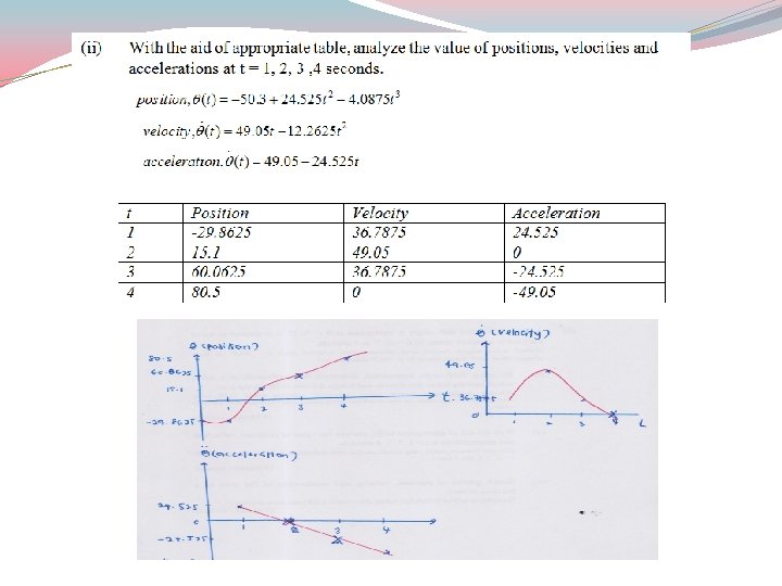
Exercise 2 – Final 2018 A single-link robot with rotary is motionless at θ = 30. 13°. It is desired to move the joint in a smooth matter to θ = 155. 28° in 4 seconds. a)By using third order polynomial, determine the coefficients of a cubic which accomplishes this motion and brings the arm to rest at the goal. b) With the aid of appropriate table, analyze the value of positions, velocities and accelerations at t = 1, 2, 3 , 4 seconds. c) Sketch graphs of position, velocity and acceleration of the joint as a function of time.

Fifth-Order Polynomial Trajectory Planning • Specify the initial and ending accelerations for a segment • To use a fifth-order polynomial for planning a trajectory, the total number of boundary conditions is 6. Calculation of the coefficients of a fifth-order polynomial with position, velocity and a acceleration boundary conditions can be possible with below equations. Initial Condition First derivative Second derivative

Cont… Constraints

Cont… Coefficients

Example �A single-link robot with a rotary join is motionless at θ=125 degrees. It is desired to move the joint to θ=67 degrees in 6 seconds. By using fifth-order polynomial, find the coefficients and plot the position, velocity and acceleration of the joint.

Final exam 2017

Answer

Final exam 2018

Final exam 2019