Plotting Linear Main Effects Models Interpreting 1 st

Plotting Linear Main Effects Models • • Interpreting 1 st order terms w/ & w/o interactions Coding & centering… gotta? oughta? Plotting single-predictor models – Q, 2 & k Plotting 2 -predictor models – 2 x. Q, kx. Q & Qx. Q

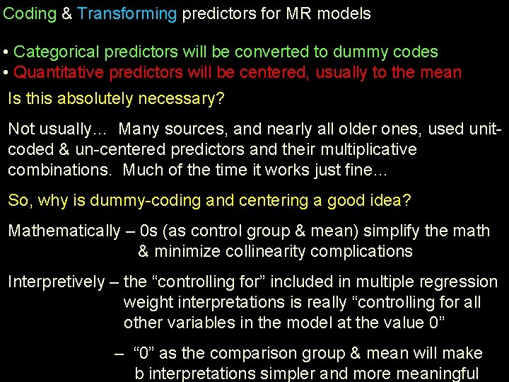
Coding & Transforming predictors for MR models • Categorical predictors will be converted to dummy codes • Quantitative predictors will be centered, usually to the mean Is this absolutely necessary? Not usually… Many sources, and nearly all older ones, used unitcoded & un-centered predictors and their multiplicative combinations. Much of the time it works just fine… So, why is dummy-coding and centering a good idea? Mathematically – 0 s (as control group & mean) simplify the math & minimize collinearity complications Interpretively – the “controlling for” included in multiple regression weight interpretations is really “controlling for all other variables in the model at the value 0” – “ 0” as the comparison group & mean will make b interpretations simpler and more meaningful

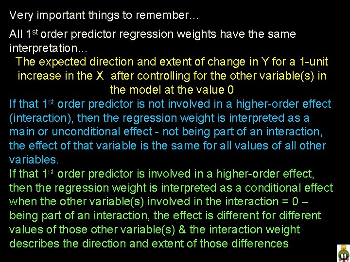
Very important things to remember… All 1 st order predictor regression weights have the same interpretation… The expected direction and extent of change in Y for a 1 -unit increase in the X after controlling for the other variable(s) in the model at the value 0 If that 1 st order predictor is not involved in a higher-order effect (interaction), then the regression weight is interpreted as a main or unconditional effect - not being part of an interaction, the effect of that variable is the same for all values of all other variables. If that 1 st order predictor is involved in a higher-order effect, then the regression weight is interpreted as a conditional effect when the other variable(s) involved in the interaction = 0 – being part of an interaction, the effect is different for different values of those other variable(s) & the interaction weight describes the direction and extent of those differences

Plotting Single-Predictor models Let’s start by getting, interpreting and plotting a model with each of the different kinds of predictor we will be working with… Be sure to “get” how each regression weight represents a particular slope, height or height differences in the plot!!!

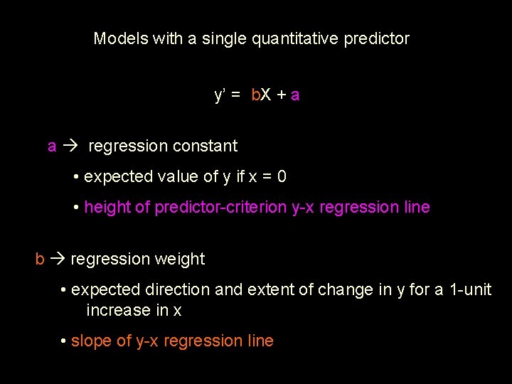
Models with a single quantitative predictor y’ = b. X + a a regression constant • expected value of y if x = 0 • height of predictor-criterion y-x regression line b regression weight • expected direction and extent of change in y for a 1 -unit increase in x • slope of y-x regression line

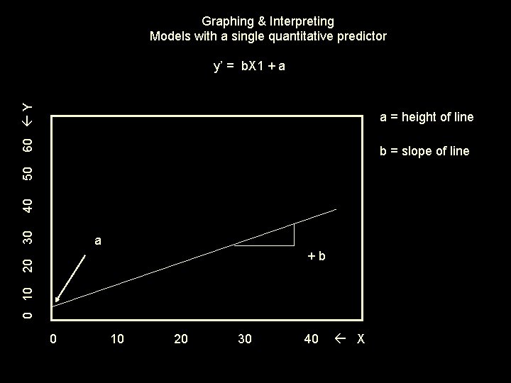
Graphing & Interpreting Models with a single quantitative predictor 60 Y y’ = b. X 1 + a a = height of line 30 40 50 b = slope of line a 0 10 20 +b 0 10 20 30 40 X

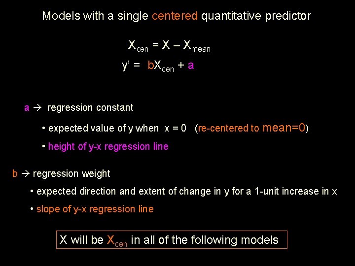
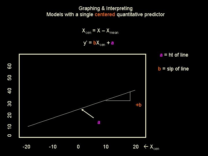
Models with a single centered quantitative predictor Xcen = X – Xmean y’ = b. Xcen + a a regression constant • expected value of y when x = 0 (re-centered to mean=0) • height of y-x regression line b regression weight • expected direction and extent of change in y for a 1 -unit increase in x • slope of y-x regression line X will be Xcen in all of the following models

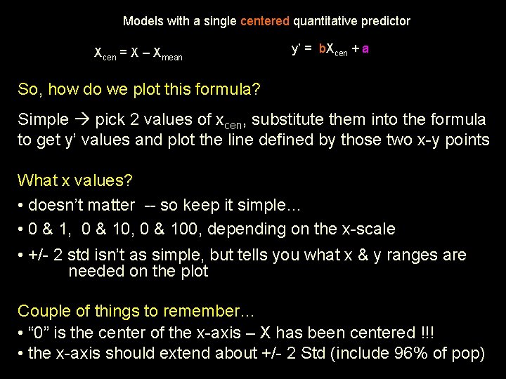
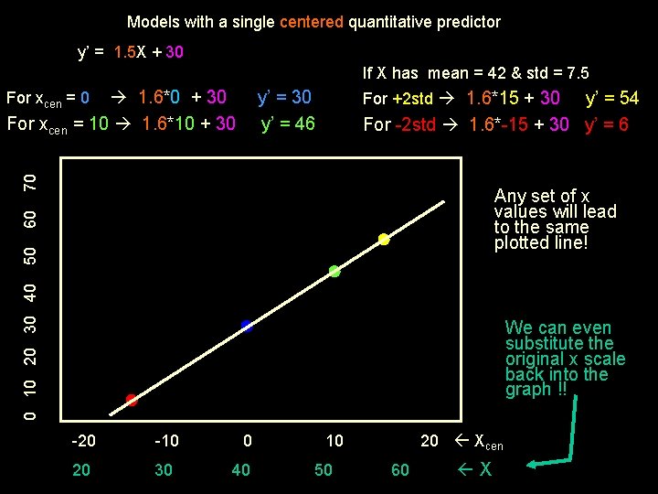
Models with a single centered quantitative predictor Xcen = X – Xmean y’ = b. Xcen + a So, how do we plot this formula? Simple pick 2 values of xcen, substitute them into the formula to get y’ values and plot the line defined by those two x-y points What x values? • doesn’t matter -- so keep it simple… • 0 & 1, 0 & 100, depending on the x-scale • +/- 2 std isn’t as simple, but tells you what x & y ranges are needed on the plot Couple of things to remember… • “ 0” is the center of the x-axis – X has been centered !!! • the x-axis should extend about +/- 2 Std (include 96% of pop)

Models with a single centered quantitative predictor y’ = 1. 5 X + 30 If X has mean = 42 & std = 7. 5 1. 6*0 + 30 For xcen = 10 1. 6*10 + 30 y’ = 46 For +2 std 1. 6*15 + 30 y’ = 54 For -2 std 1. 6*-15 + 30 y’ = 6 70 For xcen = 0 0 10 20 30 40 50 60 Any set of x values will lead to the same plotted line! We can even substitute the original x scale back into the graph !! -20 -10 20 30 0 40 10 50 20 Xcen 60 X

Graphing & Interpreting Models with a single centered quantitative predictor Xcen = X – Xmean y’ = b. Xcen + a 60 a = ht of line 30 40 50 b = slp of line 20 +b 0 10 a -20 -10 0 10 20 Xcen

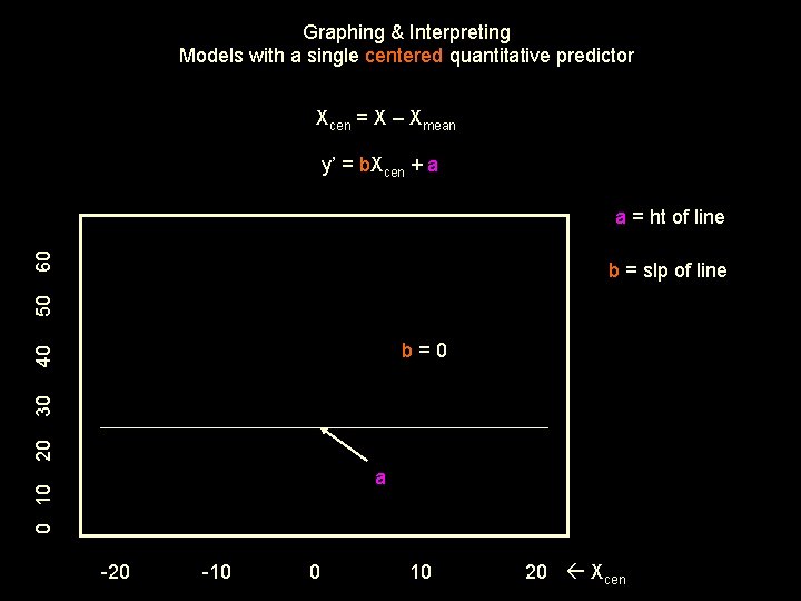
Graphing & Interpreting Models with a single centered quantitative predictor Xcen = X – Xmean y’ = b. Xcen + a 60 a = ht of line 50 b = slp of line 20 30 40 b=0 0 10 a -20 -10 0 10 20 Xcen

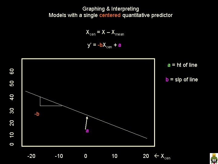
Graphing & Interpreting Models with a single centered quantitative predictor Xcen = X – Xmean y’ = -b. Xcen + a 60 a = ht of line -b 20 30 40 50 b = slp of line 0 10 a -20 -10 0 10 20 Xcen

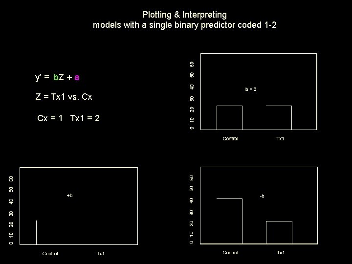
Plotting & Interpreting models with a single binary predictor coded 1 -2 y’ = b. Z + a Z = Tx 1 vs. Cx Cx = 1 Tx 1 = 2

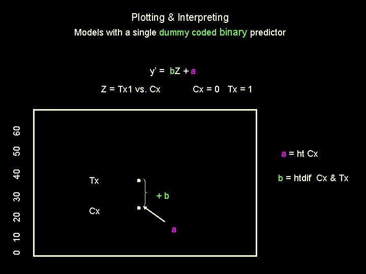
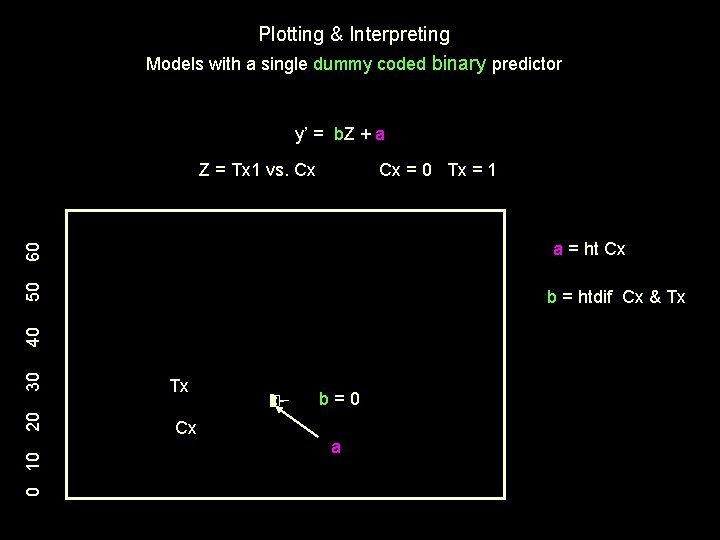
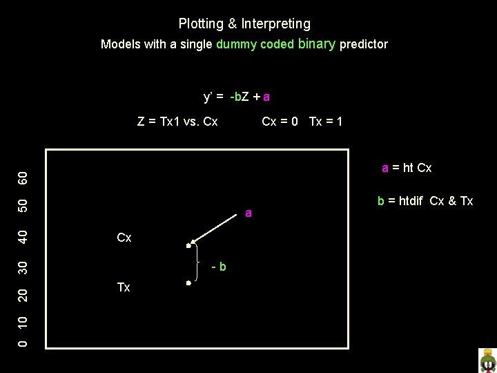
Models with a single dummy coded binary predictor y’ = b. Z + a a regression constant • expected value of y if z = 0 (the control group) • mean of the control group • height of control group b regression weight • expected direction and extent of change in y for a 1 -unit increase in x • direction and extent of y mean difference between groups coded 0 & 1 • group height difference The way we’re going to graph this model looks strange, but will provide simplicity & clarity for more complex models.

Plotting & Interpreting Models with a single dummy coded binary predictor y’ = b. Z + a Cx = 0 Tx = 1 a = ht Cx 20 0 10 b = htdif Cx & Tx Tx +b 30 40 50 60 Z = Tx 1 vs. Cx Cx a

Plotting & Interpreting Models with a single dummy coded binary predictor y’ = b. Z + a Z = Tx 1 vs. Cx Cx = 0 Tx = 1 50 60 a = ht Cx 0 10 20 30 40 b = htdif Cx & Tx Tx Cx b=0 a

Plotting & Interpreting Models with a single dummy coded binary predictor y’ = -b. Z + a Z = Tx 1 vs. Cx Cx = 0 Tx = 1 a Cx -b 0 10 20 30 40 50 60 a = ht Cx Tx b = htdif Cx & Tx

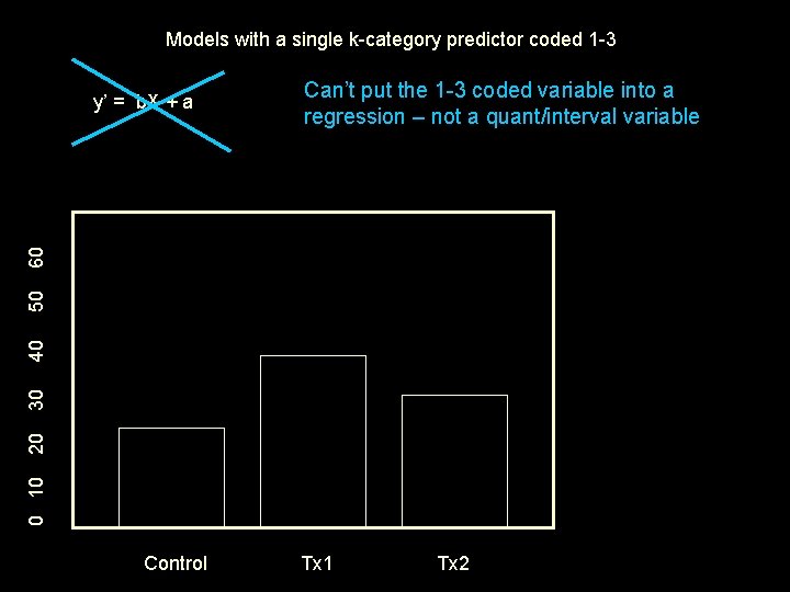
Models with a single k-category predictor coded 1 -3 Can’t put the 1 -3 coded variable into a regression – not a quant/interval variable 0 10 20 30 40 50 60 y’ = b. X + a Control Tx 1 Tx 2

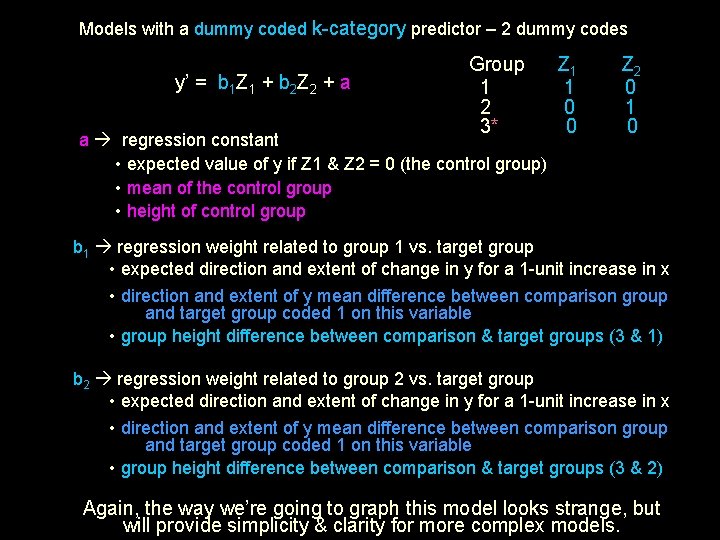
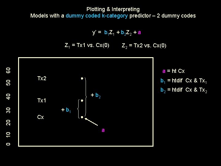
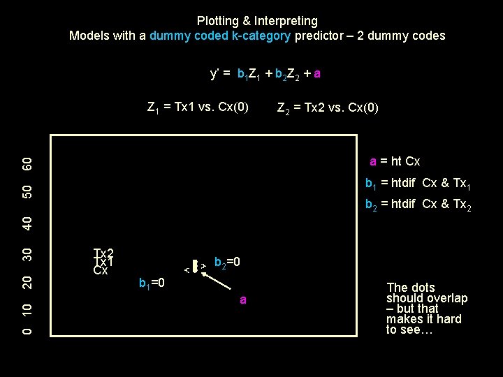
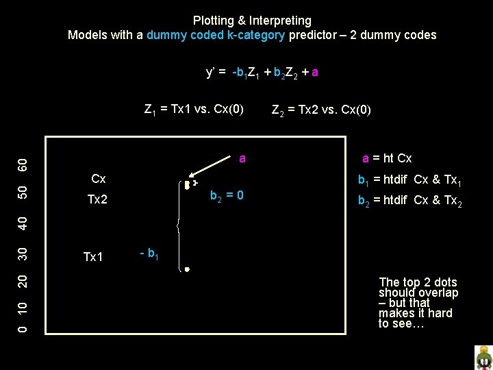
Models with a dummy coded k-category predictor – 2 dummy codes y’ = b 1 Z 1 + b 2 Z 2 + a Group 1 2 3* a regression constant • expected value of y if Z 1 & Z 2 = 0 (the control group) • mean of the control group • height of control group Z 1 1 0 0 Z 2 0 1 0 b 1 regression weight related to group 1 vs. target group • expected direction and extent of change in y for a 1 -unit increase in x • direction and extent of y mean difference between comparison group and target group coded 1 on this variable • group height difference between comparison & target groups (3 & 1) b 2 regression weight related to group 2 vs. target group • expected direction and extent of change in y for a 1 -unit increase in x • direction and extent of y mean difference between comparison group and target group coded 1 on this variable • group height difference between comparison & target groups (3 & 2) Again, the way we’re going to graph this model looks strange, but will provide simplicity & clarity for more complex models.

Plotting & Interpreting Models with a dummy coded k-category predictor – 2 dummy codes y’ = b 1 Z 1 + b 2 Z 2 + a 20 0 10 Z 2 = Tx 2 vs. Cx(0) a = ht Cx Tx 2 b 1 = htdif Cx & Tx 1 b 2 = htdif Cx & Tx 2 + b 2 Tx 1 + b 1 30 40 50 60 Z 1 = Tx 1 vs. Cx(0) Cx a

Plotting & Interpreting Models with a dummy coded k-category predictor – 2 dummy codes y’ = b 1 Z 1 + b 2 Z 2 + a Z 1 = Tx 1 vs. Cx(0) Z 2 = Tx 2 vs. Cx(0) 60 a = ht Cx 50 b 1 = htdif Cx & Tx 1 0 10 20 30 40 b 2 = htdif Cx & Tx 2 Tx 1 Cx b 2=0 b 1=0 a The dots should overlap – but that makes it hard to see…

Plotting & Interpreting Models with a dummy coded k-category predictor – 2 dummy codes y’ = -b 1 Z 1 + b 2 Z 2 + a a Cx b 2 = 0 Tx 2 Z 2 = Tx 2 vs. Cx(0) a = ht Cx b 1 = htdif Cx & Tx 1 b 2 = htdif Cx & Tx 2 0 10 20 30 40 50 60 Z 1 = Tx 1 vs. Cx(0) Tx 1 - b 1 The top 2 dots should overlap – but that makes it hard to see…

Plotting 2 -Predictor Linear Main Effects Models Now we get to the fun part – plotting multiple regression equations involving multiple variables. Three kinds (for now, more later) … • centered quant variable & dummy-coded binary variable • centered quant variable & dummy-coded k-category variable • 2 centered quant variables What we’re trying to do is to plot these models so that we can see how both of the predictors are related to the criterion. Like when we’re plotting data from a factorial design, we have to represent 3 variables -- the criterion & the 2 predictors X & Z -- in a 2 -dimensional plot. We’ll use the same solution. . We’ll plot the relationship between one predictor and the criterion for different values of the other predictor

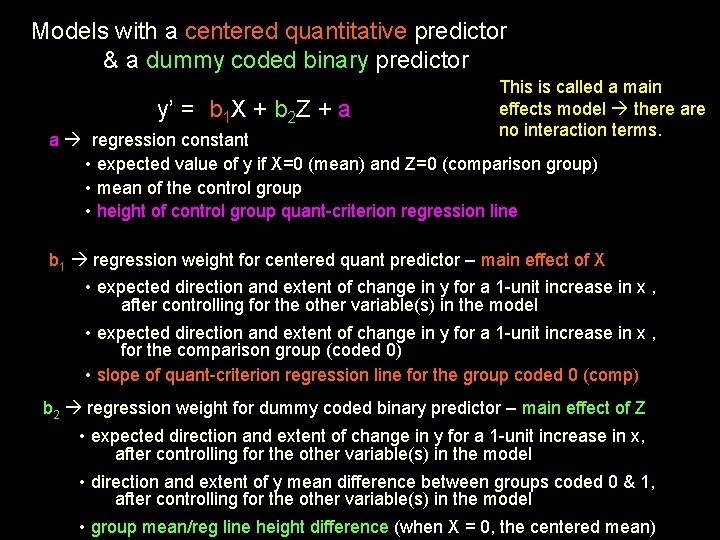
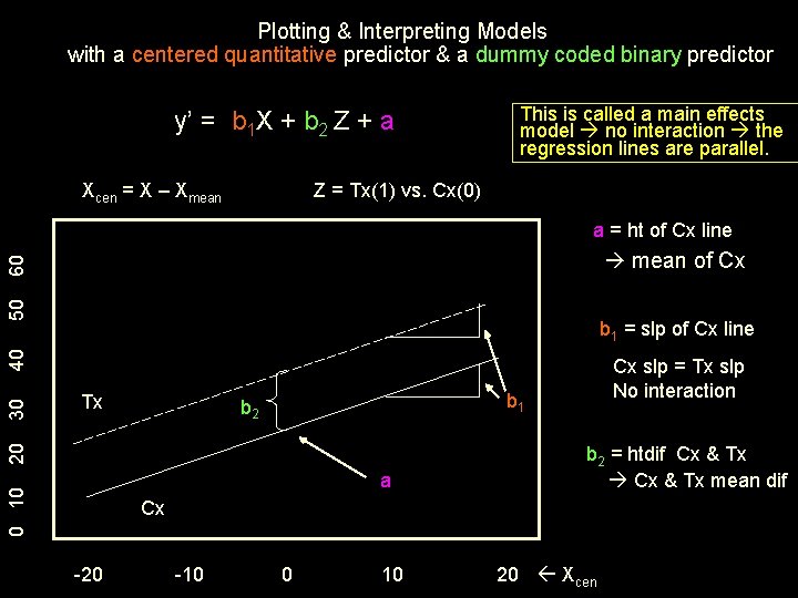
Models with a centered quantitative predictor & a dummy coded binary predictor y’ = b 1 X + b 2 Z + a This is called a main effects model there are no interaction terms. a regression constant • expected value of y if X=0 (mean) and Z=0 (comparison group) • mean of the control group • height of control group quant-criterion regression line b 1 regression weight for centered quant predictor – main effect of X • expected direction and extent of change in y for a 1 -unit increase in x , after controlling for the other variable(s) in the model • expected direction and extent of change in y for a 1 -unit increase in x , for the comparison group (coded 0) • slope of quant-criterion regression line for the group coded 0 (comp) b 2 regression weight for dummy coded binary predictor – main effect of Z • expected direction and extent of change in y for a 1 -unit increase in x, after controlling for the other variable(s) in the model • direction and extent of y mean difference between groups coded 0 & 1, after controlling for the other variable(s) in the model • group mean/reg line height difference (when X = 0, the centered mean)

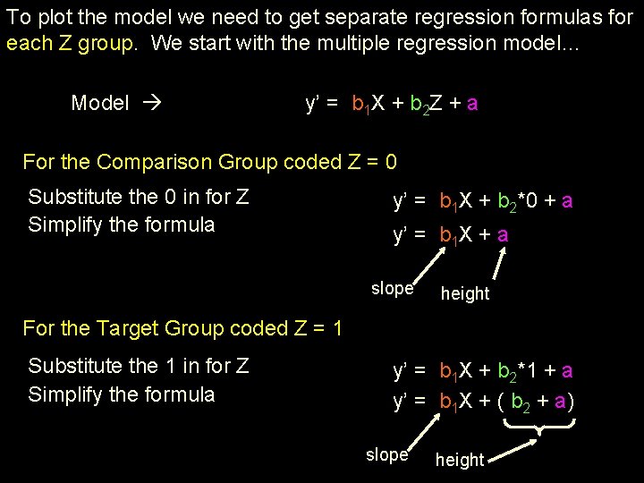
To plot the model we need to get separate regression formulas for each Z group. We start with the multiple regression model… Model y’ = b 1 X + b 2 Z + a For the Comparison Group coded Z = 0 Substitute the 0 in for Z Simplify the formula y’ = b 1 X + b 2*0 + a y’ = b 1 X + a slope height For the Target Group coded Z = 1 Substitute the 1 in for Z Simplify the formula y’ = b 1 X + b 2*1 + a y’ = b 1 X + ( b 2 + a) slope height

Plotting & Interpreting Models with a centered quantitative predictor & a dummy coded binary predictor y’ = b 1 X + b 2 Z + a Xcen = X – Xmean This is called a main effects model no interaction the regression lines are parallel. Z = Tx(1) vs. Cx(0) a = ht of Cx line 50 60 mean of Cx Tx a 0 10 Cx slp = Tx slp No interaction b 1 b 2 20 30 40 b 1 = slp of Cx line b 2 = htdif Cx & Tx mean dif Cx -20 -10 0 10 20 Xcen

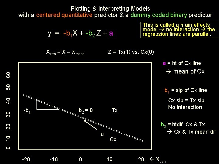
Plotting & Interpreting Models with a centered quantitative predictor & a dummy coded binary predictor y’ = -b 1 X + -b 2 Z + a Xcen = X – Xmean This is called a main effects model no interaction the regression lines are parallel. Z = Tx(1) vs. Cx(0) a = ht of Cx line 50 60 mean of Cx b 1 = slp of Cx line -b 1 b 2 = 0 Tx b 2 = htdif Cx & Tx mean dif 20 30 40 Cx slp = Tx slp No interaction 0 10 a -20 -10 0 Cx 10 20 Xcen

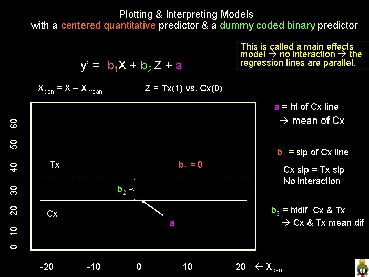
Plotting & Interpreting Models with a centered quantitative predictor & a dummy coded binary predictor y’ = b 1 X + b 2 Z + a Xcen = X – Xmean This is called a main effects model no interaction the regression lines are parallel. Z = Tx(1) vs. Cx(0) a = ht of Cx line b 1 = slp of Cx line Tx b 1 = 0 Cx -20 b 2 = htdif Cx & Tx mean dif a 0 10 20 Cx slp = Tx slp No interaction b 2 30 40 50 60 mean of Cx -10 0 10 20 Xcen

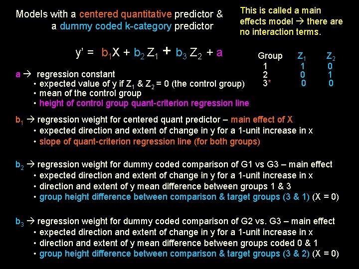
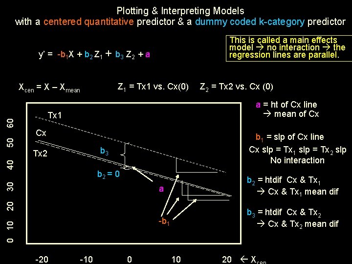
Models with a centered quantitative predictor & a dummy coded k-category predictor This is called a main effects model there are no interaction terms. y’ = b 1 X + b 2 Z 1 + b 3 Z 2 + a a regression constant • expected value of y if Z 1 & Z 2 = 0 (the control group) • mean of the control group • height of control group quant-criterion regression line Group 1 2 3* Z 1 1 0 0 Z 2 0 1 0 b 1 regression weight for centered quant predictor – main effect of X • expected direction and extent of change in y for a 1 -unit increase in x • slope of quant-criterion regression line (for both groups) b 2 regression weight for dummy coded comparison of G 1 vs G 3 – main effect • expected direction and extent of change in y for a 1 -unit increase in x • direction and extent of y mean difference between groups 1 & 3 • group height difference between comparison & target groups (3 & 1) (X = 0) b 3 regression weight for dummy coded comparison of G 2 vs. G 3 – main effect • expected direction and extent of change in y for a 1 -unit increase in x • direction and extent of y mean difference between groups coded 0 & 1 • group height difference between comparison & target groups (3 & 2) (X = 0)

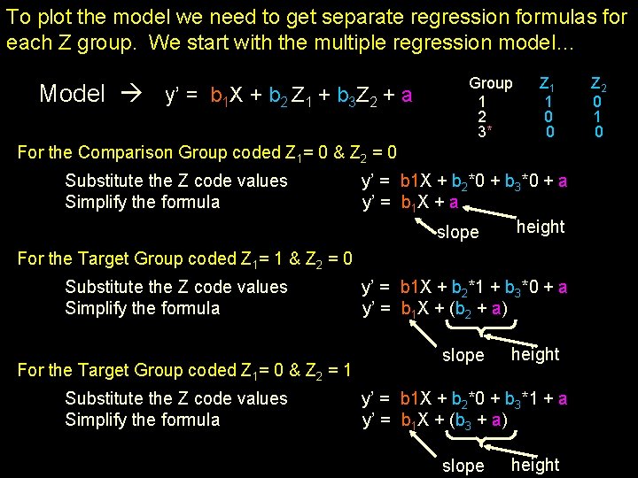
To plot the model we need to get separate regression formulas for each Z group. We start with the multiple regression model… Model y’ = b 1 X + b 2 Z 1 + b 3 Z 2 + a Group 1 2 3* Z 1 1 0 0 For the Comparison Group coded Z 1= 0 & Z 2 = 0 Substitute the Z code values Simplify the formula y’ = b 1 X + b 2*0 + b 3*0 + a y’ = b 1 X + a height slope For the Target Group coded Z 1= 1 & Z 2 = 0 Substitute the Z code values Simplify the formula For the Target Group coded Z 1= 0 & Z 2 = 1 Substitute the Z code values Simplify the formula y’ = b 1 X + b 2*1 + b 3*0 + a y’ = b 1 X + (b 2 + a) slope height y’ = b 1 X + b 2*0 + b 3*1 + a y’ = b 1 X + (b 3 + a) slope height Z 2 0 1 0

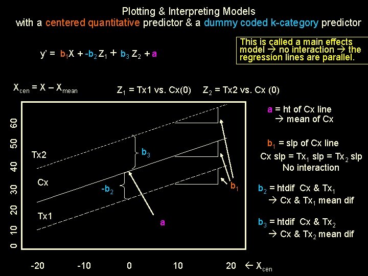
Plotting & Interpreting Models with a centered quantitative predictor & a dummy coded k-category predictor This is called a main effects model no interaction the regression lines are parallel. y’ = b 1 X + -b 2 Z 1 + b 3 Z 2 + a Xcen = X – Xmean Z 1 = Tx 1 vs. Cx(0) Z 2 = Tx 2 vs. Cx (0) 50 60 a = ht of Cx line mean of Cx b 1 = slp of Cx line Cx slp = Tx 1 slp = Tx 2 slp No interaction b 3 Cx b 1 -b 2 Tx 1 -20 -10 0 b 2 = htdif Cx & Tx 1 mean dif b 3 = htdif Cx & Tx 2 mean dif a 0 10 20 30 40 Tx 2 10 20 Xcen

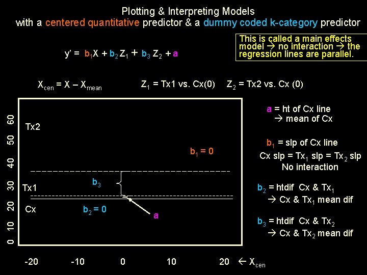
Plotting & Interpreting Models with a centered quantitative predictor & a dummy coded k-category predictor This is called a main effects model no interaction the regression lines are parallel. y’ = b 1 X + b 2 Z 1 + b 3 Z 2 + a Z 1 = Tx 1 vs. Cx(0) Z 2 = Tx 2 vs. Cx (0) a = ht of Cx line mean of Cx Tx 2 50 60 Xcen = X – Xmean 30 b 3 Cx b 2 = 0 b 2 = htdif Cx & Tx 1 mean dif a b 3 = htdif Cx & Tx 2 mean dif 0 10 Tx 1 20 40 b 1 = 0 -20 -10 b 1 = slp of Cx line Cx slp = Tx 1 slp = Tx 2 slp No interaction 0 10 20 Xcen

Plotting & Interpreting Models with a centered quantitative predictor & a dummy coded k-category predictor This is called a main effects model no interaction the regression lines are parallel. y’ = -b 1 X + b 2 Z 1 + b 3 Z 2 + a Z 1 = Tx 1 vs. Cx(0) Tx 1 Cx b 1 = slp of Cx line Cx slp = Tx 1 slp = Tx 2 slp No interaction b 3 40 Tx 2 a b 2 = htdif Cx & Tx 1 mean dif -b 1 b 3 = htdif Cx & Tx 2 mean dif 0 10 20 30 b 2 = 0 -20 Z 2 = Tx 2 vs. Cx (0) a = ht of Cx line mean of Cx 50 60 Xcen = X – Xmean -10 0 10 20 X

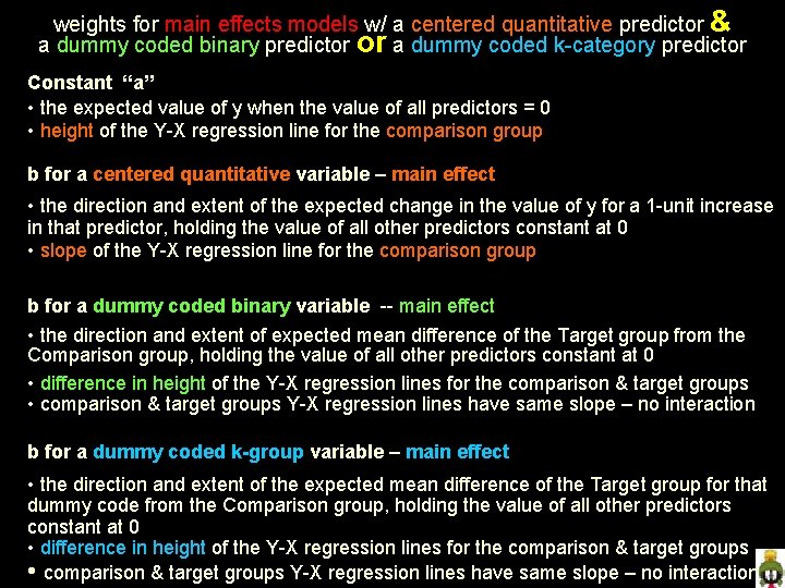
weights for main effects models w/ a centered quantitative predictor & a dummy coded binary predictor or a dummy coded k-category predictor Constant “a” • the expected value of y when the value of all predictors = 0 • height of the Y-X regression line for the comparison group b for a centered quantitative variable – main effect • the direction and extent of the expected change in the value of y for a 1 -unit increase in that predictor, holding the value of all other predictors constant at 0 • slope of the Y-X regression line for the comparison group b for a dummy coded binary variable -- main effect • the direction and extent of expected mean difference of the Target group from the Comparison group, holding the value of all other predictors constant at 0 • difference in height of the Y-X regression lines for the comparison & target groups • comparison & target groups Y-X regression lines have same slope – no interaction b for a dummy coded k-group variable – main effect • the direction and extent of the expected mean difference of the Target group for that dummy code from the Comparison group, holding the value of all other predictors constant at 0 • difference in height of the Y-X regression lines for the comparison & target groups • comparison & target groups Y-X regression lines have same slope – no interaction

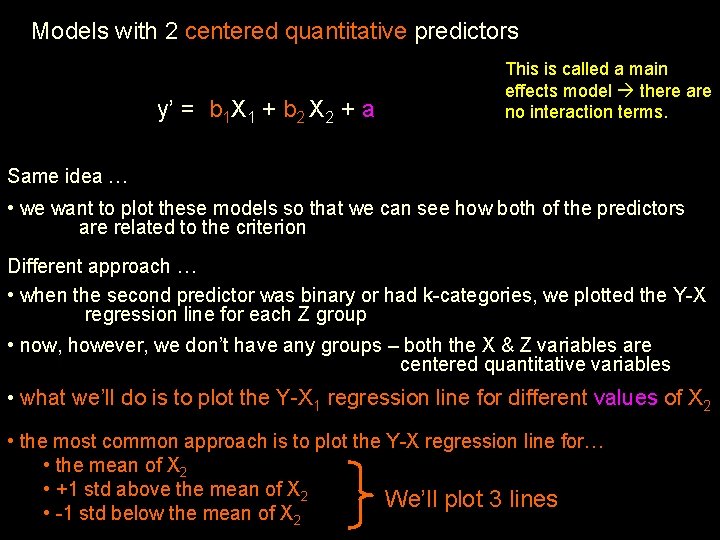
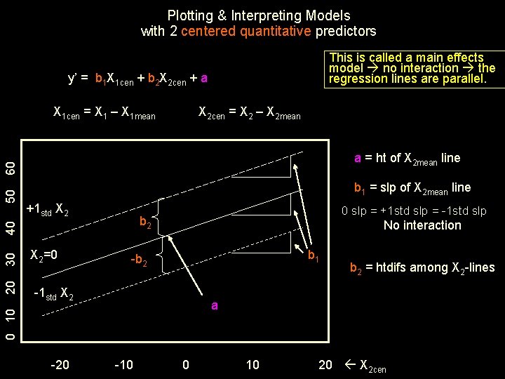
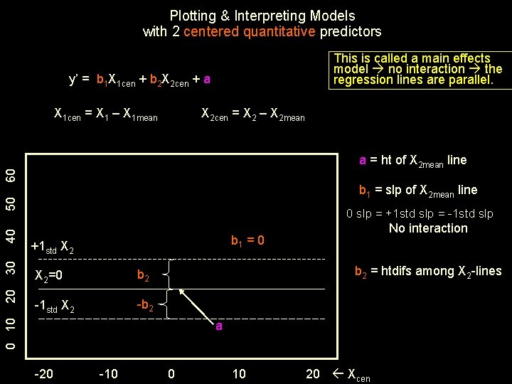
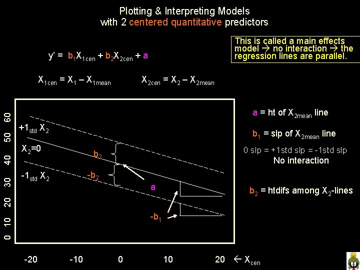
Models with 2 centered quantitative predictors y’ = b 1 X 1 + b 2 X 2 + a This is called a main effects model there are no interaction terms. Same idea … • we want to plot these models so that we can see how both of the predictors are related to the criterion Different approach … • when the second predictor was binary or had k-categories, we plotted the Y-X regression line for each Z group • now, however, we don’t have any groups – both the X & Z variables are centered quantitative variables • what we’ll do is to plot the Y-X 1 regression line for different values of X 2 • the most common approach is to plot the Y-X regression line for… • the mean of X 2 • +1 std above the mean of X 2 We’ll plot 3 lines • -1 std below the mean of X 2

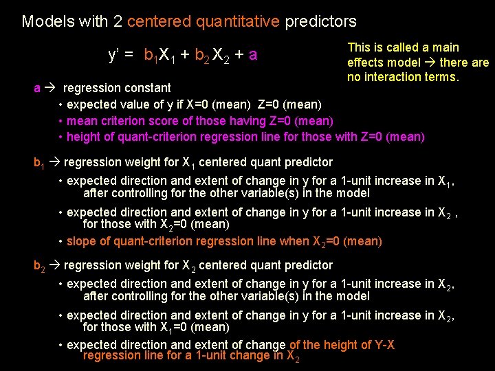
Models with 2 centered quantitative predictors y’ = b 1 X 1 + b 2 X 2 + a This is called a main effects model there are no interaction terms. a regression constant • expected value of y if X=0 (mean) Z=0 (mean) • mean criterion score of those having Z=0 (mean) • height of quant-criterion regression line for those with Z=0 (mean) b 1 regression weight for X 1 centered quant predictor • expected direction and extent of change in y for a 1 -unit increase in X 1, after controlling for the other variable(s) in the model • expected direction and extent of change in y for a 1 -unit increase in X 2 , for those with X 2=0 (mean) • slope of quant-criterion regression line when X 2=0 (mean) b 2 regression weight for X 2 centered quant predictor • expected direction and extent of change in y for a 1 -unit increase in X 2, after controlling for the other variable(s) in the model • expected direction and extent of change in y for a 1 -unit increase in X 2, for those with X 1=0 (mean) • expected direction and extent of change of the height of Y-X regression line for a 1 -unit change in X 2

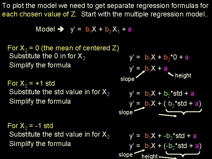
To plot the model we need to get separate regression formulas for each chosen value of Z. Start with the multiple regression model. . Model y’ = b 1 X + b 2 X 1 + a For X 2 = 0 (the mean of centered Z) Substitute the 0 in for X 2 Simplify the formula For X 2 = +1 std Substitute the std value in for X 2 Simplify the formula y’ = b 1 X + b 2*0 + a y’ = b 1 X + a slope height y’ = b 1 X + b 2*std + a y’ = b 1 X + ( b 2*std + a) slope For X 2 = -1 std Substitute the std value in for X 2 Simplify the formula y’ = b 1 X + -b 2*std + a y’ = b 1 X + (-b 2*std + a) slope height

Plotting & Interpreting Models with 2 centered quantitative predictors This is called a main effects model no interaction the regression lines are parallel. y’ = b 1 X 1 cen + b 2 X 2 cen + a X 1 cen = X 1 – X 1 mean X 2 cen = X 2 – X 2 mean b 1 = slp of X 2 mean line +1 std X 2 30 No interaction b 1 -b 2 -1 std X 2 -20 b 2 = htdifs among X 2 -lines a 0 10 20 X 2=0 0 slp = +1 std slp = -1 std slp b 2 40 50 60 a = ht of X 2 mean line -10 0 10 20 X 2 cen

Plotting & Interpreting Models with 2 centered quantitative predictors This is called a main effects model no interaction the regression lines are parallel. y’ = b 1 X 1 cen + b 2 X 2 cen + a X 1 cen = X 1 – X 1 mean X 2 cen = X 2 – X 2 mean 60 a = ht of X 2 mean line 0 slp = +1 std slp = -1 std slp No interaction b 1 = 0 +1 std X 2=0 b 2 -1 std X 2 -b 2 = htdifs among X 2 -lines 0 10 20 30 40 50 b 1 = slp of X 2 mean line a -20 -10 0 10 20 Xcen

Plotting & Interpreting Models with 2 centered quantitative predictors This is called a main effects model no interaction the regression lines are parallel. y’ = b 1 X 1 cen + b 2 X 2 cen + a X 2 cen = X 2 – X 2 mean a = ht of X 2 mean line +1 std X 2 b 1 = slp of X 2 mean line X 2=0 0 slp = +1 std slp = -1 std slp b 2 No interaction -b 2 -1 std X 2 a b 2 = htdifs among X 2 -lines 20 30 40 50 60 X 1 cen = X 1 – X 1 mean 0 10 -b 1 -20 -10 0 10 20 Xcen