Plotting choropleth maps in R with tmap Using




![ESRI shapefiles • Examine the shapefile: > shp[, 5: 7]. . . NUTS 3 ESRI shapefiles • Examine the shapefile: > shp[, 5: 7]. . . NUTS 3](https://slidetodoc.com/presentation_image_h/2d3ea3c136861c507e35915119df5f3e/image-8.jpg)






![Plotting Stat. Bank data • Plot the data t <- tm_shape(shp[shp$Statistic == stat, ]) Plotting Stat. Bank data • Plot the data t <- tm_shape(shp[shp$Statistic == stat, ])](https://slidetodoc.com/presentation_image_h/2d3ea3c136861c507e35915119df5f3e/image-20.jpg)


- Slides: 22

Plotting choropleth maps in R with tmap Using CSO ESRI shapefiles and Stat. Bank data Eoin Horgan

Table of Contents 1. Introduction 2. Mapping in R 3. Importing and mapping Stat. Bank data 2

Section 1: Introduction

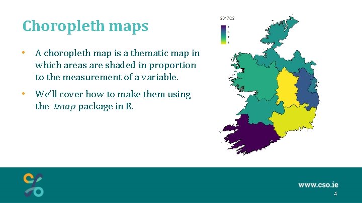
Choropleth maps • A choropleth map is a thematic map in which areas are shaded in proportion to the measurement of a variable. • We’ll cover how to make them using the tmap package in R. 4

Section 2: Mapping in R

ESRI shapefiles • Install the sf package (only necessary first time using the package) install. packages("sf") • Now we need to load the package before we can use it in this session (necessary once for every R session) library(sf) • See http: //rpubs. com/eoin-horgan-cso/tmap_code_snippets for copy/pasteable code 6

ESRI shapefiles • Covers entire country in varying granularity • Census 2011 files: • http: //census. cso. ie/censusasp/saps/boundaries/ED_SA%2 0 Disclaimer 1. htm • Load data into variable shp: shp <- st_read("shapefile. shp", strings. As. Factors = F) • Note: file is in zip archive, can use tempdir() for unzipping 7
![ESRI shapefiles Examine the shapefile shp 5 7 NUTS 3 ESRI shapefiles • Examine the shapefile: > shp[, 5: 7]. . . NUTS 3](https://slidetodoc.com/presentation_image_h/2d3ea3c136861c507e35915119df5f3e/image-8.jpg)
ESRI shapefiles • Examine the shapefile: > shp[, 5: 7]. . . NUTS 3 NAME GEOGID geometry 1 IE 024 South-East (IE) R 6 MULTIPOLYGON (((226795. 5 90. . . 2 IE 025 South-West (IE) R 7 MULTIPOLYGON (((18146. 05 95. . . 3 IE 011 Border R 1 MULTIPOLYGON (((306570. 4 30. . . 4 IE 012 Midland R 5 MULTIPOLYGON (((223420. 6 29. . . 5 IE 013 West R 8 MULTIPOLYGON (((48596. 74 26. . . … 8

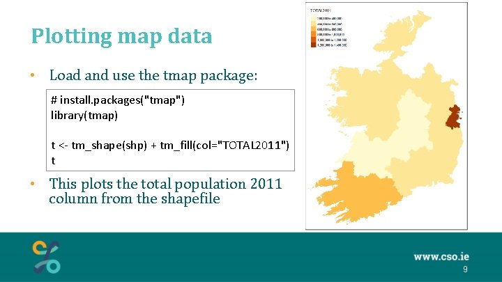
Plotting map data • Load and use the tmap package: # install. packages("tmap") library(tmap) t <- tm_shape(shp) + tm_fill(col="TOTAL 2011") t • This plots the total population 2011 column from the shapefile 9

Customising map appearance • Colour palette: t <- tm_shape(shp) + tm_fill(col="TOTAL 2011", palette = viridis. Lite: : viridis(20), color. NA = "grey 50", legend. reverse = TRUE, title = "Population 2011") t • See library(tmaptools); palette_explorer() for all colour palettes • http: //sape. inf. usi. ch/sites/default/files/ggplot 2 -colour-names. png for R colours 10

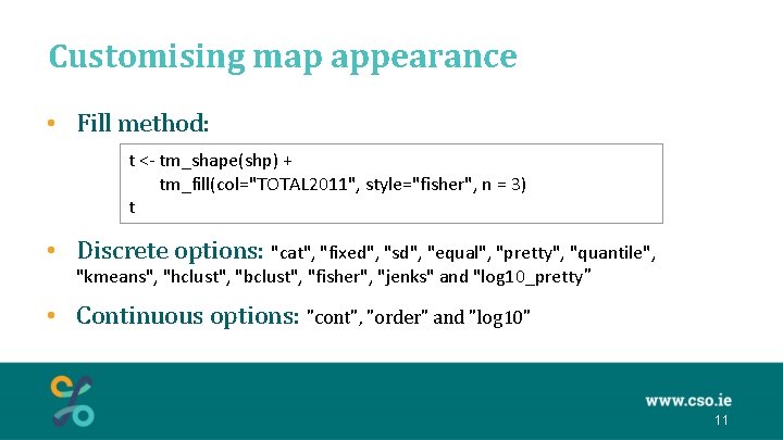
Customising map appearance • Fill method: t <- tm_shape(shp) + tm_fill(col="TOTAL 2011", style="fisher", n = 3) t • Discrete options: "cat", "fixed", "sd", "equal", "pretty", "quantile", "kmeans", "hclust", "bclust", "fisher", "jenks" and "log 10_pretty" • Continuous options: "cont", "order" and "log 10" 11

Customising map appearance • Borders t <- tm_shape(shp) + tm_fill(col="TOTAL 2011") + tm_borders(col = "black", lwd = 1) t • Again, colour can be any of the standard R colours 12

Customising map appearance • Other options: • Remove frame, increase legend size t <- tm_shape(shp) + tm_fill(col="TOTAL 2011", palette = viridis. Lite: : viridis(20), style="cont", legend. reverse = TRUE, title = "Population 2011") + tm_borders(col = "black") + tm_layout(frame = FALSE, scale = 1. 6) t 13

Section 3: Importing and mapping Stat. Bank data

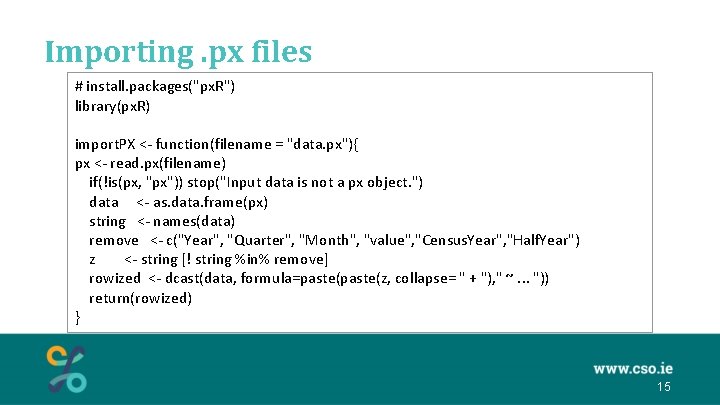
Importing. px files # install. packages("px. R") library(px. R) import. PX <- function(filename = "data. px"){ px <- read. px(filename) if(!is(px, "px")) stop("Input data is not a px object. ") data <- as. data. frame(px) string <- names(data) remove <- c("Year", "Quarter", "Month", "value", "Census. Year", "Half. Year") z <- string [! string %in% remove] rowized <- dcast(data, formula=paste(z, collapse= " + "), " ~. . . ")) return(rowized) } 15

Importing. px files • Import table QNQ 22 as the variable df • Again, saving on local machine is faster df <- import. PX(paste 0("https: //statbank. cso. ie/px/pxeirestat/", "Database/eirestat/Quarterly%20 National%20 Household", "%20 Survey%20 Main%20 Results/QNQ 22. px")) # or df <- import. PX("C: \Users\path\to\your\file\QNQ 22. px") 16

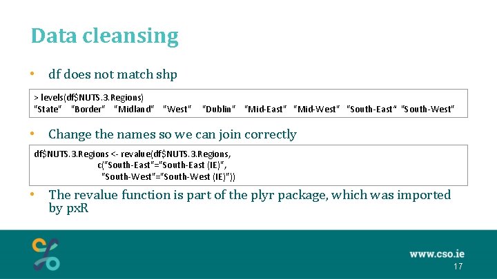
Data cleansing • df does not match shp > levels(df$NUTS. 3. Regions) "State" "Border" "Midland" "West" "Dublin" "Mid-East" "Mid-West" "South-East“ "South-West" • Change the names so we can join correctly df$NUTS. 3. Regions <- revalue(df$NUTS. 3. Regions, c("South-East"="South-East (IE)", "South-West"="South-West (IE)")) • The revalue function is part of the plyr package, which was imported by px. R 17

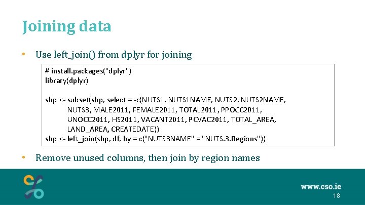
Joining data • Use left_join() from dplyr for joining # install. packages("dplyr") library(dplyr) shp <- subset(shp, select = -c(NUTS 1, NUTS 1 NAME, NUTS 2 NAME, NUTS 3, MALE 2011, FEMALE 2011, TOTAL 2011, PPOCC 2011, UNOCC 2011, HS 2011, VACANT 2011, PCVAC 2011, TOTAL_AREA, LAND_AREA, CREATEDATE)) shp <- left_join(shp, df, by = c("NUTS 3 NAME" = "NUTS. 3. Regions")) • Remove unused columns, then join by region names 18

Plotting Stat. Bank data • Choose statistic and year to display var <- "2017 Q 2" # Choose from "1997 Q 4" to "2017 Q 2" stat <- as. character(levels(shp$Statistic)[4]) # Choose from 1 to 5 # [1] Persons aged 15 years and over in Employment (Thousand) # [2] Unemployed Persons aged 15 years and over (Thousand) # [3] Persons aged 15 years and over in Labour Force (Thousand) # [4] ILO Unemployment Rate (15 - 74 years) (%) # [5] ILO Participation Rate (15 years and over) (%) 19
![Plotting Stat Bank data Plot the data t tmshapeshpshpStatistic stat Plotting Stat. Bank data • Plot the data t <- tm_shape(shp[shp$Statistic == stat, ])](https://slidetodoc.com/presentation_image_h/2d3ea3c136861c507e35915119df5f3e/image-20.jpg)
Plotting Stat. Bank data • Plot the data t <- tm_shape(shp[shp$Statistic == stat, ]) + tm_fill(col=var, palette = viridis. Lite: : viridis(20), style = "cont", color. NA = "grey 50", title = "ILO Unemployment Rate (%), n(15 - 74 years), 2017 Q 2", popup. vars=c("GEOGID", var)) + tm_borders(col = "black") + tm_layout(frame = FALSE, scale = 1. 1, legend. width = 0. 7) t 20

Interactivity • Change to interactive mode tmap_mode("view") t • Return to plotting mode tmap_mode("plot") t 21
