Plotting and Models Biology 683 Heath Blackmon Remember
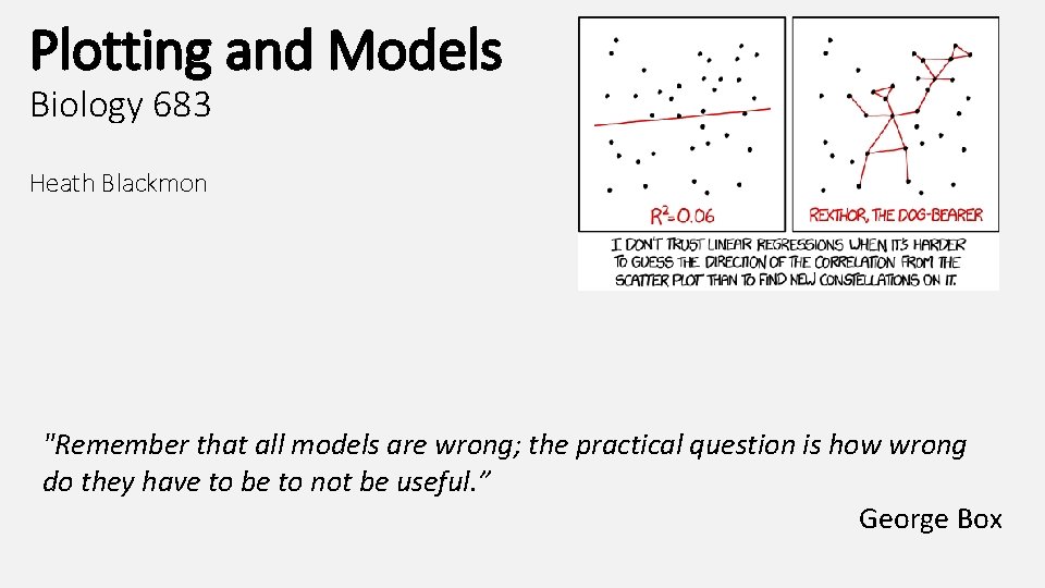
Plotting and Models Biology 683 Heath Blackmon "Remember that all models are wrong; the practical question is how wrong do they have to be to not be useful. ” George Box
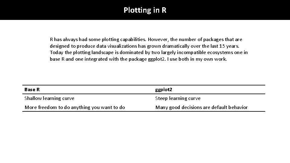
Plotting in R R has always had some plotting capabilities. However, the number of packages that are designed to produce data visualizations has grown dramatically over the last 15 years. Today the plotting landscape is dominated by two largely incompatible ecosystems one in base R and one integrated with the package ggplot 2. I use both in my own work. Base R ggplot 2 Shallow learning curve Steep learning curve More freedom to do anything you want to do Many good decisions are default behavior
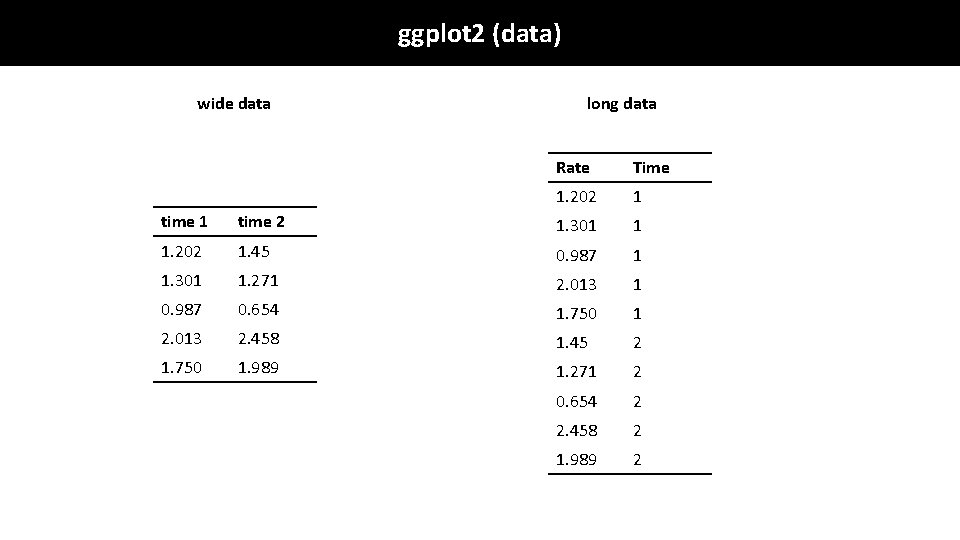
ggplot 2 (data) wide data long data Rate Time 1. 202 1 time 2 1. 301 1 1. 202 1. 45 0. 987 1 1. 301 1. 271 2. 013 1 0. 987 0. 654 1. 750 1 2. 013 2. 458 1. 45 2 1. 750 1. 989 1. 271 2 0. 654 2 2. 458 2 1. 989 2
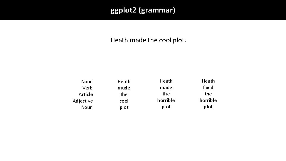
ggplot 2 (grammar) Heath made the cool plot. Noun Verb Article Adjective Noun Heath made the cool plot Heath made the horrible plot Heath fixed the horrible plot
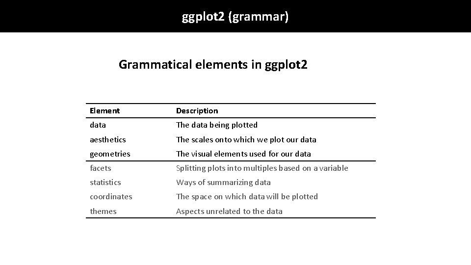
ggplot 2 (grammar) Grammatical elements in ggplot 2 Element Description data The data being plotted aesthetics The scales onto which we plot our data geometries The visual elements used for our data facets Splitting plots into multiples based on a variable statistics Ways of summarizing data coordinates The space on which data will be plotted themes Aspects unrelated to the data
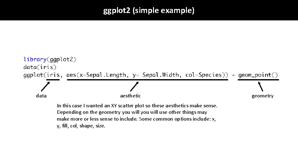
ggplot 2 (simple example) data aesthetic In this case I wanted an XY scatter plot so these aesthetics make sense. Depending on the geometry you will use other things may make more or less sense to include. Some common options include: x, y, fill, col, shape, size. geometry
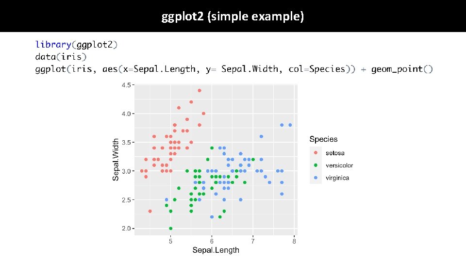
ggplot 2 (simple example)
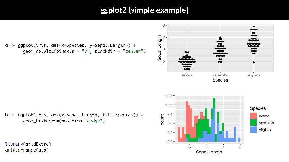
ggplot 2 (simple example)
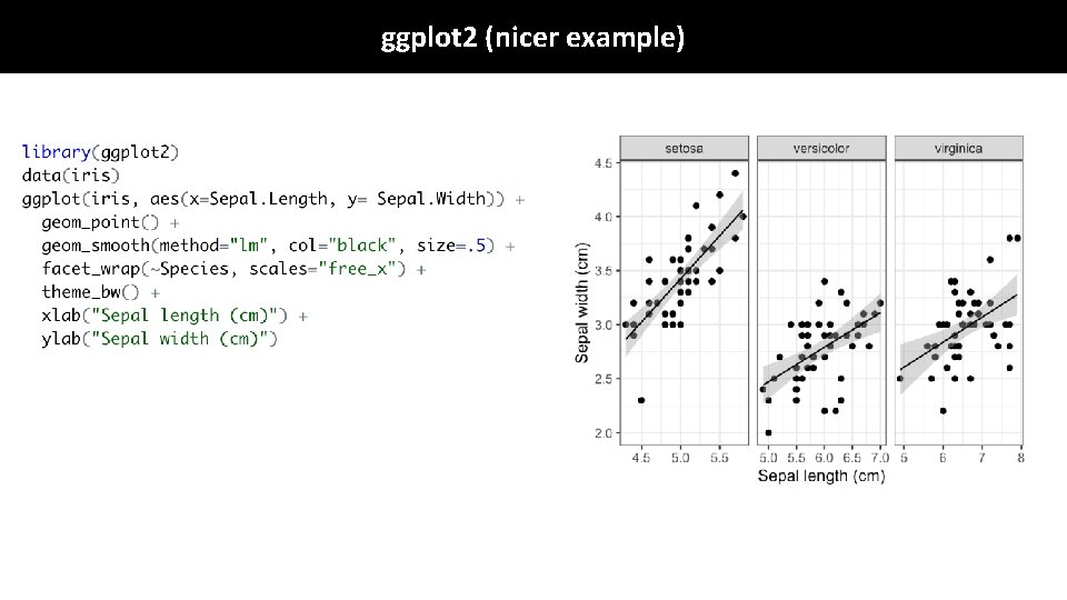
ggplot 2 (nicer example)
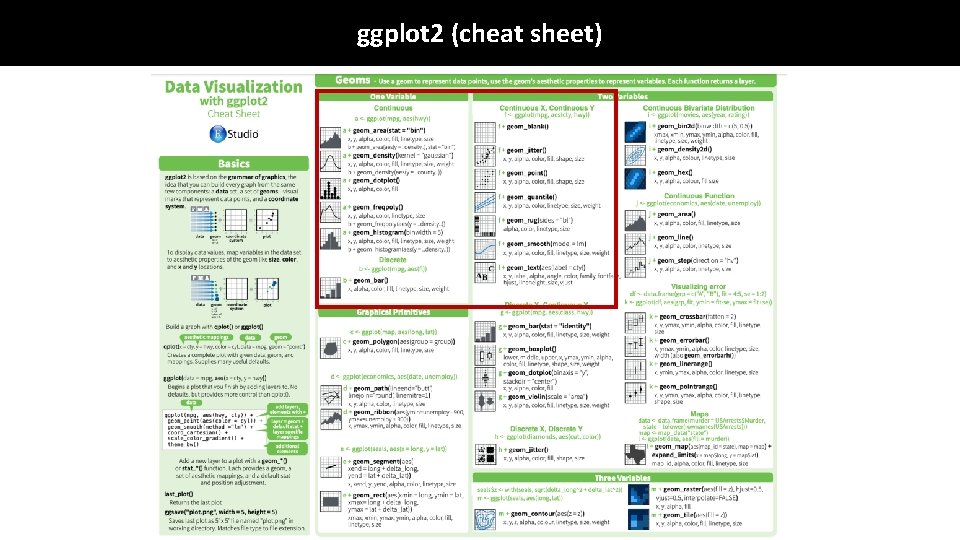
ggplot 2 (cheat sheet)
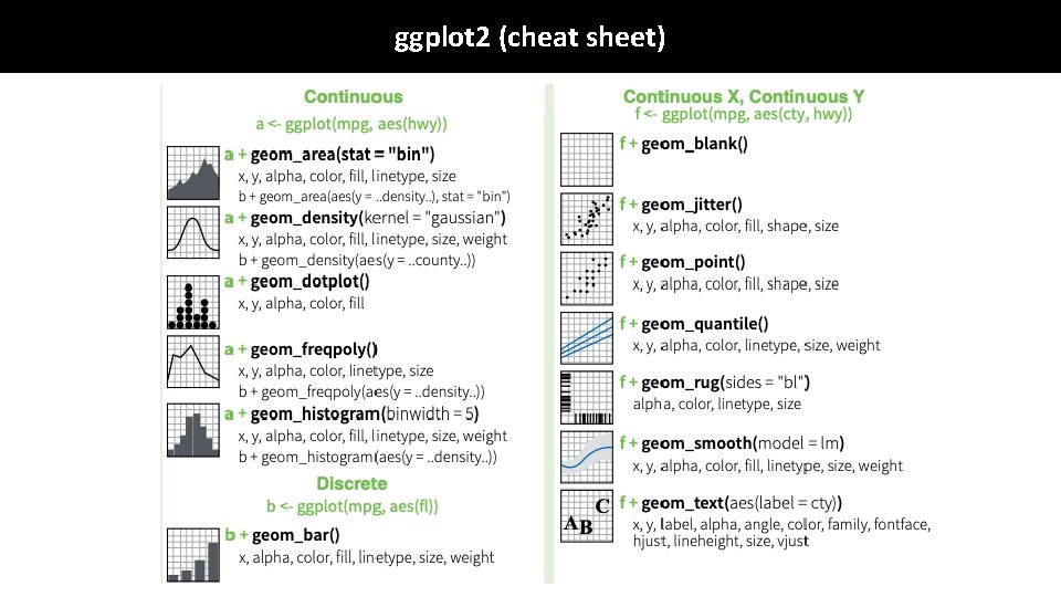
ggplot 2 (cheat sheet)
ggrapt. R – a gentle transition to ggplot
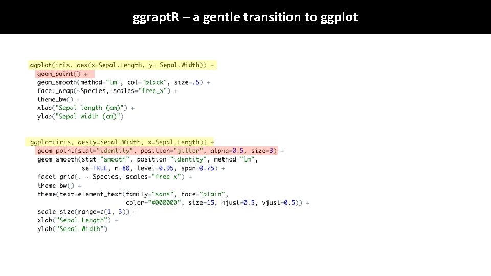
ggrapt. R – a gentle transition to ggplot

Homework Using the betta data and ggplot 2 make an awesome plot that includes 3 variables (2 numerical and 1 discrete) – Due by Tuesday class time.

Correlation vs Regression • Both methods are ways to explore contingency between variables. • Regression describes the degree to which we can predict the value of one variable based on the value of another. • Regression calculates a line that describes this relationship between two variables. • Use regression when you believe there is a strong case for causation.
Correlation vs Regression • Both methods are ways to explore contingency between variables. • Regression describes the degree to which we can predict the value of one variable based on the value of another. • Regression calculates a line that describes this relationship between two variables. • Use regression when you believe there is a strong case for causation.
Terminology Linear regression vs. OLS regression (Ordinary least squares regression) vs. General linear models vs. Generalized linear model
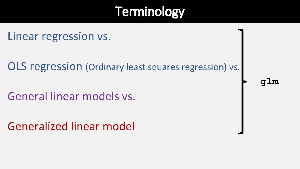
Terminology Linear regression vs. OLS regression (Ordinary least squares regression) vs. glm General linear models vs. Generalized linear model
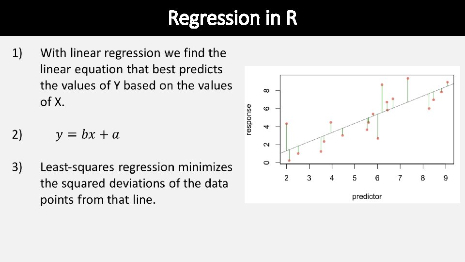
Regression in R
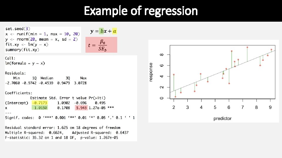
Example of regression
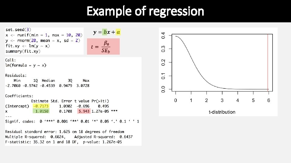
Example of regression
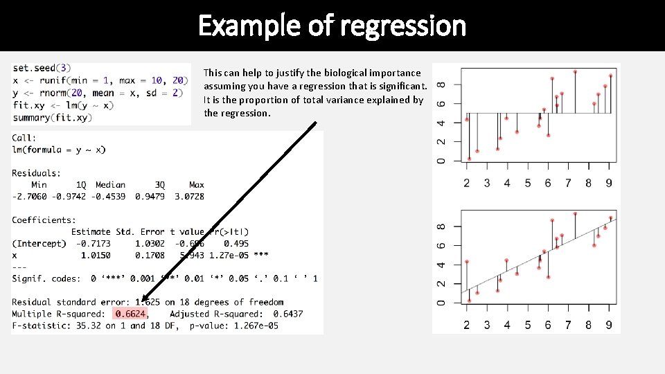
Example of regression This can help to justify the biological importance assuming you have a regression that is significant. It is the proportion of total variance explained by the regression.
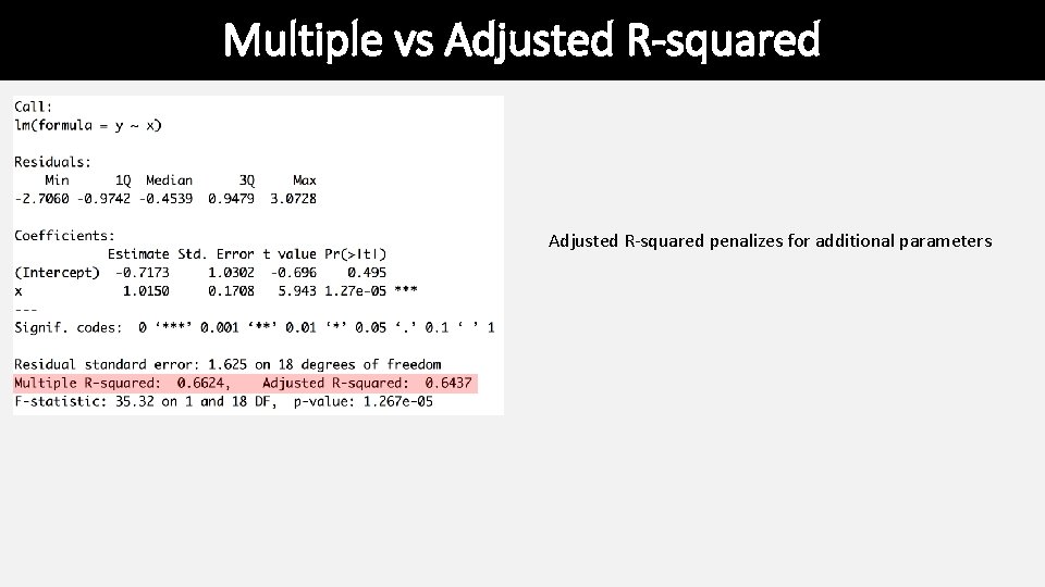
Multiple vs Adjusted R-squared penalizes for additional parameters
Linear regression uses • Depict the relationship between two variables in an eye-catching fashion • Test the null hypothesis of no association between two variables • The test is whether or not the slope is zero • Predict the average value of variable Y for a group of individuals with a given value of variable X • • variation around the line can make it very difficult to predict a value for a given individual with much confidence Predictions outside of the range of observed data is generally discouraged • Used both for experimental and observational studies
What are Residuals In general, the residual is the individual’s departure from the value predicted by the model In this case the model is simple – the linear regression – but residuals also exist for more complex models For a model that fits better, the residuals will be smaller on average Residuals can be of interest in their own right, because they represent values that have been corrected for relationships that might be obscuring a pattern.
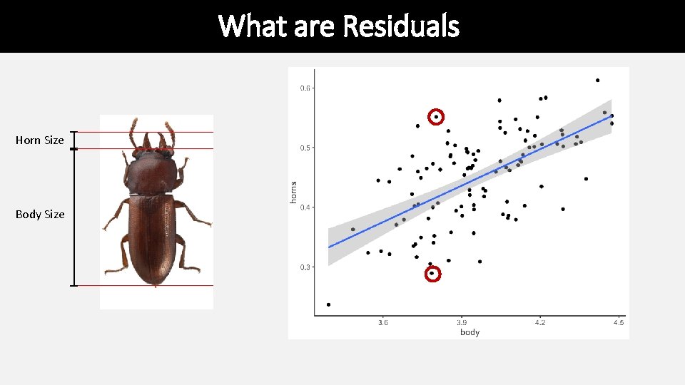
What are Residuals Horn Size Body Size
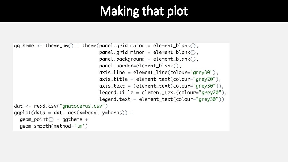
Making that plot
Strong Inference for Observational Studies • Noticing a pattern in the data and reporting it represents a post hoc analysis • This is not hypothesis testing • The results, while potentially important, must be interpreted cautiously What can be done? • Based on a post-hoc observational study, construct a new hypothesis for a novel group or system that has not yet been studied
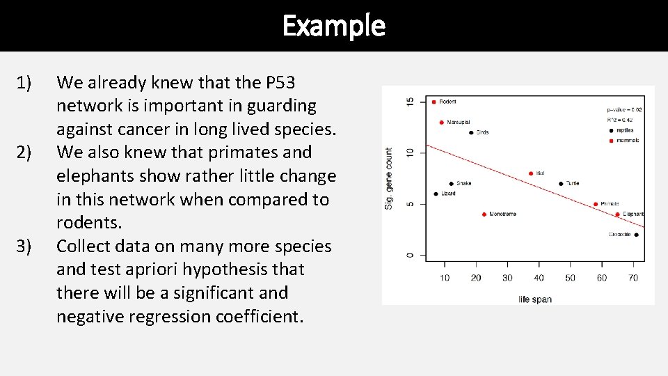
Example 1) 2) 3) We already knew that the P 53 network is important in guarding against cancer in long lived species. We also knew that primates and elephants show rather little change in this network when compared to rodents. Collect data on many more species and test apriori hypothesis that there will be a significant and negative regression coefficient.
Assumptions of Linear Regression • The true relationship must be linear • At each value of X, the distribution of Y is normal (i. e. , the residuals are normal) • The variance in Y is independent of the value of X • Note that there are no assumptions about the distribution of X
Common Problems • Outliers • • • Regression is extremely sensitive to outliers The line will be drawn to outliers, especially along the x-axis Consider performing the regression with and without outliers • Non-linearity • • Best way to notice is by visually inspecting the plot and the line fit Try a transformation to get linearity [often a log transformation] • Non-normality of residuals • • Can be detected from a residual plot Possibly solved with a transformation • Unequal variance • Usually visible from a scatterplot or from a residual plot
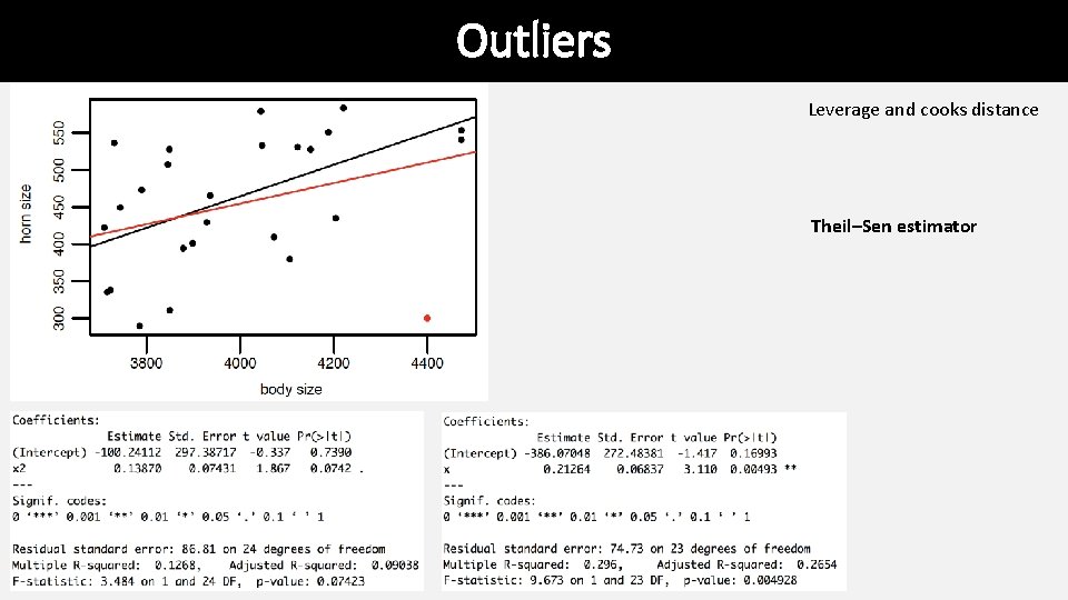
Outliers Leverage and cooks distance Theil–Sen estimator
Moving past simple models • The reason ANOVA is so widely used is that it provides a framework to simultaneously test the effects of multiple factors • ANOVA also makes it possible to detect interactions among the factors • ANOVA is a special case of a general linear model • Linear regression is a special case of a general linear model
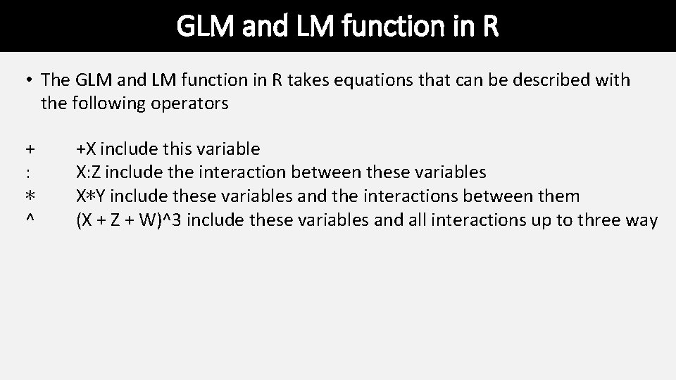
GLM and LM function in R • The GLM and LM function in R takes equations that can be described with the following operators + : ∗ ^ +X include this variable X: Z include the interaction between these variables X∗Y include these variables and the interactions between them (X + Z + W)^3 include these variables and all interactions up to three way
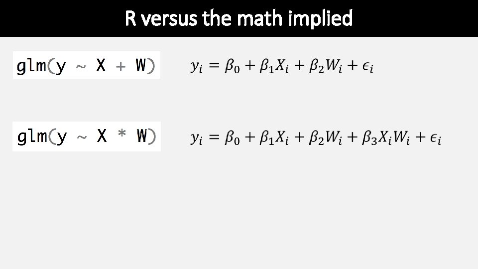
R versus the math implied
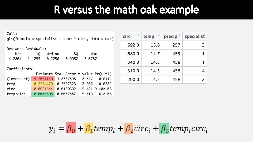
R versus the math oak example
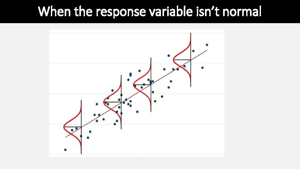
When the response variable isn’t normal
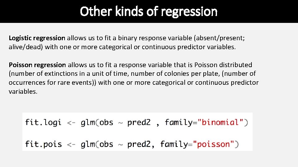
Other kinds of regression Logistic regression allows us to fit a binary response variable (absent/present; alive/dead) with one or more categorical or continuous predictor variables. Poisson regression allows us to fit a response variable that is Poisson distributed (number of extinctions in a unit of time, number of colonies per plate, (number of occurrences for rare events)) with one or more categorical or continuous predictor variables.
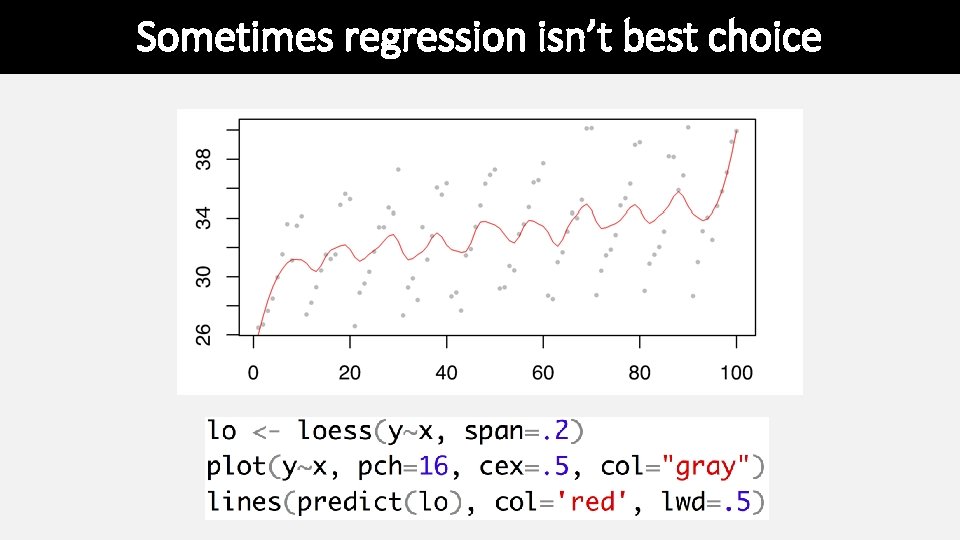
Sometimes regression isn’t best choice
- Slides: 39