Plot functions Plot a function with single variable

Plot functions • Plot a function with single variable • Syntax: function[x_]: =; Plot[f[x], {{x, xinit, xlast}}]; Plot[{f 1[x], f 2[x]}, {x, xinit, xlast}]; • Plot various single-variable functions in Chapter 1, ZCA 110 as examples. • Plot a few functions on the same graph.

Plot a few functions on the same graph • F 1[x_]: =1*x; • F 2[x_]: =2*x; • F 3[x_]: =3*x; • F 4[x_]: =4*x; • list={F 1[x], F 2[x], F 3[x], F 4[x]}; • Plot[list, {x, -10, 10}]

Plot a few functions on the same graphs • Do the same thing by defining the functions to depend on x and n: • F[x_, n_]: =n*x; • list={F[x, 1], F[x, 2], F[x, 3], F[x, 4]}; • Plot[list, {x, -10, 10}]

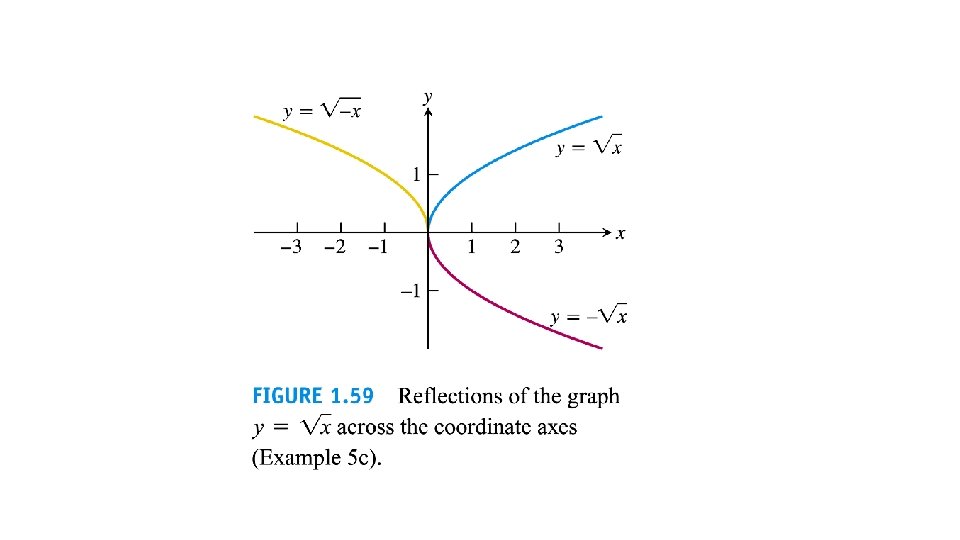
Black Body Radiation

Exercise • Plot Planck’s law of black body radiation for various temperatures on the same graph by defining R as a function of two variables. • Define function of two variables: • h, c, T, are constants; • R[lambda_, T_]: =2 Pi*h*c^2/(lambda^5*(Exp[h*c/(lambda*k*T)]-1)); • Customize the plots using these: • Plot. Label; Axes. Label; Plot. Legend; Plot. Range;

Exercise: •

Syntax: Table[]; Sum[] •

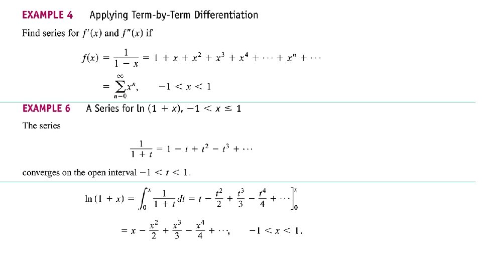
Example 2 Finding Taylor polynomial for ex at x = 0 10

Exercise: Numerical verification of • Expectation value of a photon’s energy when deriving Planck’s law for black body radiation; • Define • The sum over all n in the RHS should converge to in the limit n infinity. 11

Constructing wave pulse • Two pure waves with slight difference in frequency and wave number Dw = w 1 - w 2, Dk= k 1 - k 2, are superimposed 12

Envelop wave and phase wave The resultant wave is a ‘wave group’ comprise of an `envelop’ (or the group wave) and a phase waves 13

Wave pulse – an even more `localised’ wave • In the previous example, we add up only two slightly different wave to form a train of wave group • An even more `localised’ group wave – what we call a “wavepulse” can be constructed by adding more sine waves of different numbers ki and possibly different amplitudes so that they interfere constructively over a small region Dx and outside this region they interfere destructively so that the resultant field approach zero • Mathematically, 14

A wavepulse – the wave is well localised within Dx. This is done by adding a lot of waves with their wave parameters {Ai, ki, wi} slightly differ from each other (i = 1, 2, 3…. as many as it can) 15

Exercise: Simulating wave group and wave pulse • Construct a code to add n waves, each with an angular frequency omegai and wave number ki into a wave pulse for a fixed t. • Display the wave pulse for t=t 0, t=t 1, …, t=tn. • Syntax: Manipulate • Sample code: wavepulse. nb

Syntax: Parametric. Plot[], Show[] •

2 D projectile motion (recall your Mechanics class) • Plot the trajectories of a 2 D projectile launched with a common initial speed but at different angles • Plot the trajectories of a 2 D projectile launched with a common angle but different initial speed. • Sample code: 2 Dprojectile. nb • For a fixed v 0 and theta, how would you determine the maximum height numerically (not using formula)?

Exercise: Circular motion • Write down the parametric equations for the x and y coordinates of an object executing circular motion. • Plot the trajectories of a particle moving in a circle (recall your vector analysis class, ZCT 211)

Parametric Equation of an Ellipse b a C(h, k) • http: //en. wikipedia. org/wiki/Semi-major_axis • In geometry, the major axis of an ellipse is its longest diameter: line segment that runs through the center and both foci, with ends at the widest points of the perimeter. The semi-major axis, a, is one half of the major axis, and thus runs from the centre, through a focus, and to the perimeter. Essentially, it is the radius of an orbit at the orbit's two most distant points. For the special case of a circle, the semi-major axis is the radius. One can think of the semi-major axis as an ellipse's long radius.

Geometry of an ellipse The distance to the focal point from the center of the ellipse is sometimes called the linear eccentricity, f, of the ellipse. In terms of semi-major and semi-minor, f 2 = a 2 −b 2. e is the eccentricity of an ellipse is the ratio of the distance between the two foci, to the length of the major axis or e = 2 f/2 a = f/a

• Elliptic orbit of a planet around the Sun C(h, k)

Exercise: Marking a point on a 2 D plane. • x = h + a cos wt; y = k + b sin wt. Set w=1. • Display the parametric plot for an ellipse with your choice of h, k, a, b. • How would you mark a point with the coordinate (x(t), y(t)) on the ellipse? • Syntax: List. Plot[{{x[t], y[t]}}]; • You can customize the size of the point using Plot. Style->Point. Size[0. 05], Plot. Markers;

Exercise: Simulating an ellipse trajectory in 2 D • How would you construct a simulation displaying a point going around the ellipse as time advances? • Sample code: ellipse 1. nb

Exercise: • (i) Given any moment t, how would you abstract the coordinates of a point P(t) on the ellipse? • (ii) How could you obtain the coordinates P’(t) at the other end of the straight line connecting to point P(t) via the center point (h, k)? (you have to think!) • (iii) Given the knowledge of P(t) and P’(t), draw a line connecting these two points on the ellipse (see sample code 3 in ellipse 1. nb) at fixed t. • (iv) Simulate the rotation of the straight line about (h, k) as the point P move around the ellipse. • (v) Use your code to “measure” the maximum and minimum distances between the points PP’ (known as major axis and minor axis). Theoretically, major axis = Max[2 b, 2 a]; minor axis = Min[2 b, 2 a]; see ellipse 2. nb

Exercise: Simulating SHM • O q L

Exercise: Simulating SHM • Simulate two SHMs with different lengths L 1, L 2: • Plot the phase difference between them as a function of time.