Plantwide control Control structure design for complete chemical

Plantwide control (Control structure design for complete chemical plants) Sigurd Skogestad Department of Chemical Engineering Norwegian University of Science and Tecnology (NTNU) Trondheim, Norway Based on: Plenary presentation at ESCAPE’ 12, May 2002 Updated/expanded April 2004 for 2. 5 h tutorial in Vancouver, Canada Further updated: August 2004, December 2004, August 2005 1

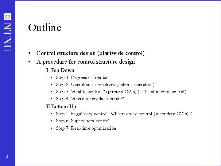
Outline • Control structure design (plantwide control) • A procedure for control structure design I Top Down • • Step 1: Degrees of freedom Step 2: Operational objectives (optimal operation) Step 3: What to control ? (primary CV’s) (self-optimizing control) Step 4: Where set production rate? II Bottom Up • Step 5: Regulatory control: What more to control (secondary CV’s) ? • Step 6: Supervisory control • Step 7: Real-time optimization 2

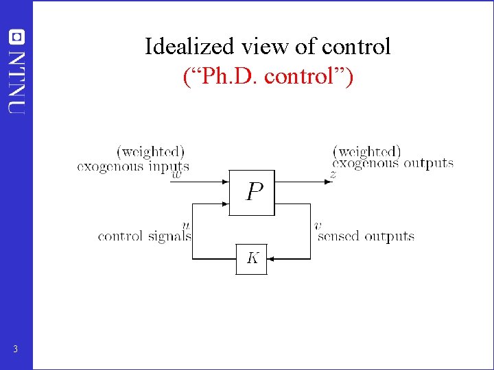
Idealized view of control (“Ph. D. control”) 3

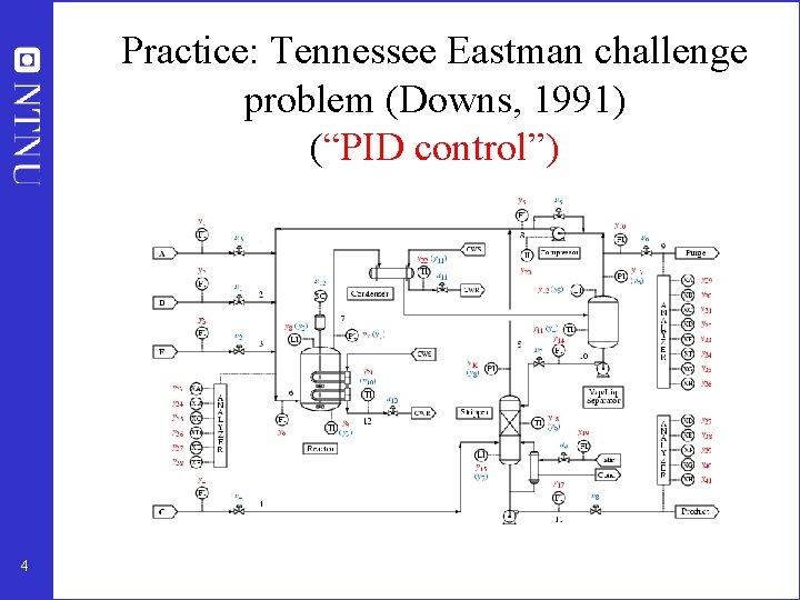
Practice: Tennessee Eastman challenge problem (Downs, 1991) (“PID control”) 4

How we design a control system for a complete chemical plant? • • 5 Where do we start? What should we control? and why? etc.

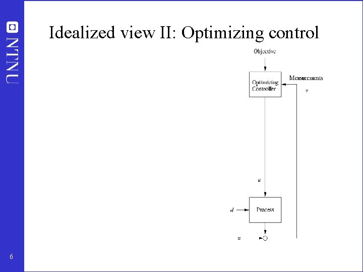
Idealized view II: Optimizing control 6

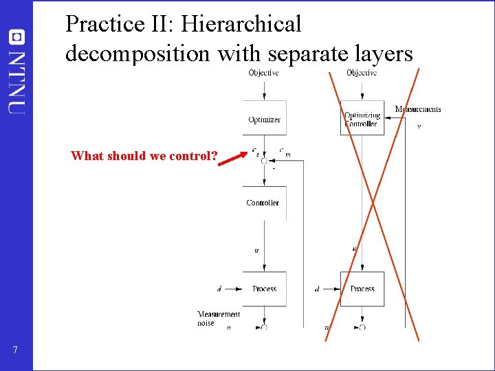
Practice II: Hierarchical decomposition with separate layers What should we control? 7

• Alan Foss (“Critique of chemical process control theory”, AICh. E Journal, 1973): The central issue to be resolved. . . is the determination of control system structure. Which variables should be measured, which inputs should be manipulated and which links should be made between the two sets? There is more than a suspicion that the work of a genius is needed here, for without it the control configuration problem will likely remain in a primitive, hazily stated and wholly unmanageable form. The gap is present indeed, but contrary to the views of many, it is theoretician who must close it. • Carl Nett (1989): Minimize control system complexity subject to the achievement of accuracy specifications in the face of uncertainty. 8

Control structure design • Not the tuning and behavior of each control loop, • But rather the control philosophy of the overall plant with emphasis on the structural decisions: – – Selection of controlled variables (“outputs”) Selection of manipulated variables (“inputs”) Selection of (extra) measurements Selection of control configuration (structure of overall controller that interconnects the controlled, manipulated and measured variables) – Selection of controller type (LQG, H-infinity, PID, decoupler, MPC etc. ). • That is: Control structure design includes all the decisions we need make to get from ``PID control’’ to “Ph. D” control 9

Process control: “Plantwide control” = “Control structure design for complete chemical plant” • • Large systems Each plant usually different – modeling expensive Slow processes – no problem with computation time Structural issues important – What to control? – Extra measurements – Pairing of loops 10

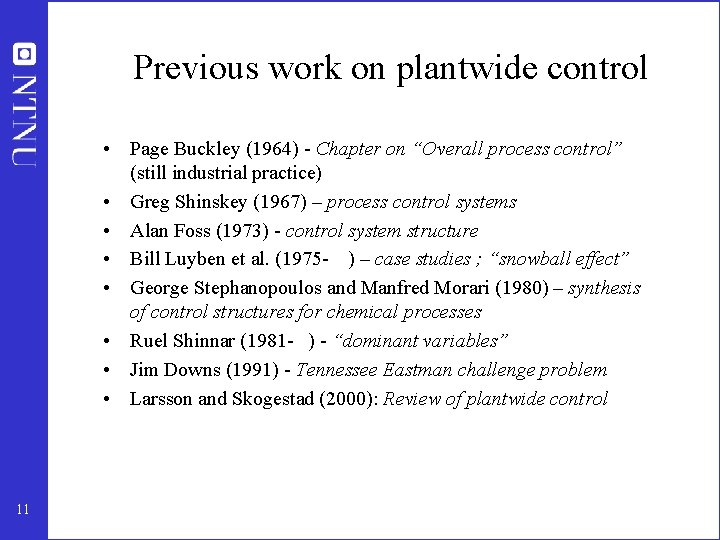
Previous work on plantwide control • Page Buckley (1964) - Chapter on “Overall process control” (still industrial practice) • Greg Shinskey (1967) – process control systems • Alan Foss (1973) - control system structure • Bill Luyben et al. (1975 - ) – case studies ; “snowball effect” • George Stephanopoulos and Manfred Morari (1980) – synthesis of control structures for chemical processes • Ruel Shinnar (1981 - ) - “dominant variables” • Jim Downs (1991) - Tennessee Eastman challenge problem • Larsson and Skogestad (2000): Review of plantwide control 11

• Control structure selection issues are identified as important also in other industries. Professor Gary Balas (Minnesota) at ECC’ 03 about flight control at Boeing: The most important control issue has always been to select the right controlled variables --- no systematic tools used! 12

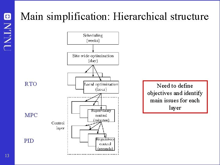
Main simplification: Hierarchical structure RTO MPC PID 13 Need to define objectives and identify main issues for each layer

Regulatory control (seconds) • Purpose: “Stabilize” the plant by controlling selected ‘’secondary’’ variables (y 2) such that the plant does not drift too far away from its desired operation • Use simple single-loop PI(D) controllers • Status: Many loops poorly tuned – Most common setting: Kc=1, I=1 min (default) – Even wrong sign of gain Kc …. 14

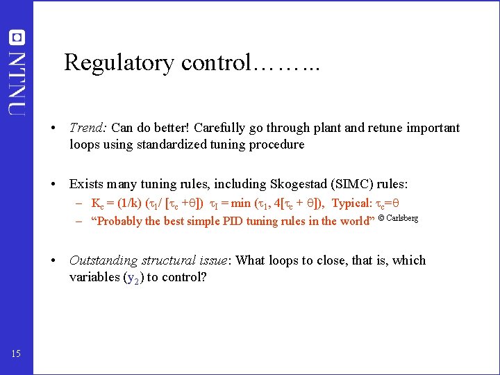
Regulatory control……. . . • Trend: Can do better! Carefully go through plant and retune important loops using standardized tuning procedure • Exists many tuning rules, including Skogestad (SIMC) rules: – Kc = (1/k) ( 1/ [ c + ]) I = min ( 1, 4[ c + ]), Typical: c= – “Probably the best simple PID tuning rules in the world” © Carlsberg • Outstanding structural issue: What loops to close, that is, which variables (y 2) to control? 15

Supervisory control (minutes) • Purpose: Keep primary controlled variables (c=y 1) at desired values, using as degrees of freedom the setpoints y 2 s for the regulatory layer. • Status: Many different “advanced” controllers, including feedforward, decouplers, overrides, cascades, selectors, Smith Predictors, etc. • Issues: – Which variables to control may change due to change of “active constraints” – Interactions and “pairing” 16

Supervisory control…. . . • Trend: Model predictive control (MPC) used as unifying tool. – Linear multivariable models with input constraints – Tuning (modelling) is time-consuming and expensive • Issue: When use MPC and when use simpler single-loop decentralized controllers ? – MPC is preferred if active constraints (“bottleneck”) change. – Avoids logic for reconfiguration of loops • Outstanding structural issue: – What primary variables c=y 1 to control? 17

Local optimization (hour) • Purpose: Minimize cost function J and: – Identify active constraints – Recompute optimal setpoints y 1 s for the controlled variables • Status: Done manually by clever operators and engineers • Trend: Real-time optimization (RTO) based on detailed nonlinear steady-state model • Issues: – Optimization not reliable. – Need nonlinear steady-state model – Modelling is time-consuming and expensive 18

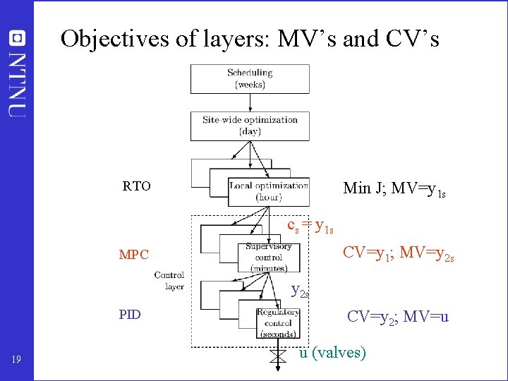
Objectives of layers: MV’s and CV’s RTO Min J; MV=y 1 s cs = y 1 s CV=y 1; MV=y 2 s MPC y 2 s PID 19 CV=y 2; MV=u u (valves)

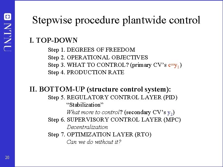
Stepwise procedure plantwide control I. TOP-DOWN Step 1. DEGREES OF FREEDOM Step 2. OPERATIONAL OBJECTIVES Step 3. WHAT TO CONTROL? (primary CV’s c=y 1) Step 4. PRODUCTION RATE II. BOTTOM-UP (structure control system): Step 5. REGULATORY CONTROL LAYER (PID) “Stabilization” What more to control? (secondary CV’s y 2) Step 6. SUPERVISORY CONTROL LAYER (MPC) Decentralization Step 7. OPTIMIZATION LAYER (RTO) Can we do without it? 20

Step 1. Degrees of freedom (DOFs) • m – dynamic (control) degrees of freedom = valves • u 0 – steady-state degrees of freedom • Cost J depends normally on steady-state DOFs 21

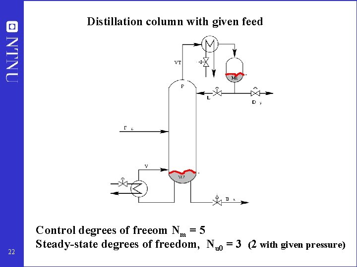
Distillation column with given feed 22 Control degrees of freeom Nm = 5 Steady-state degrees of freedom, Nu 0 = 3 (2 with given pressure)

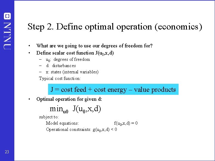
Step 2. Define optimal operation (economics) • • What are we going to use our degrees of freedom for? Define scalar cost function J(u 0, x, d) – u 0: degrees of freedom – d: disturbances – x: states (internal variables) Typical cost function: J = cost feed + cost energy – value products • Optimal operation for given d: minu 0 J(u 0, x, d) subject to: Model equations: f(u 0, x, d) = 0 Operational constraints: g(u 0, x, d) < 0 23

Step 3. What should we control (c)? • Implementation of optimal operation 24

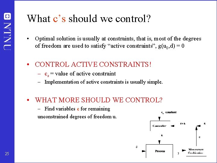
What c’s should we control? • Optimal solution is usually at constraints, that is, most of the degrees of freedom are used to satisfy “active constraints”, g(u 0, d) = 0 • CONTROL ACTIVE CONSTRAINTS! – cs = value of active constraint – Implementation of active constraints is usually simple. • WHAT MORE SHOULD WE CONTROL? – Find variables c for remaining unconstrained degrees of freedom u. 25

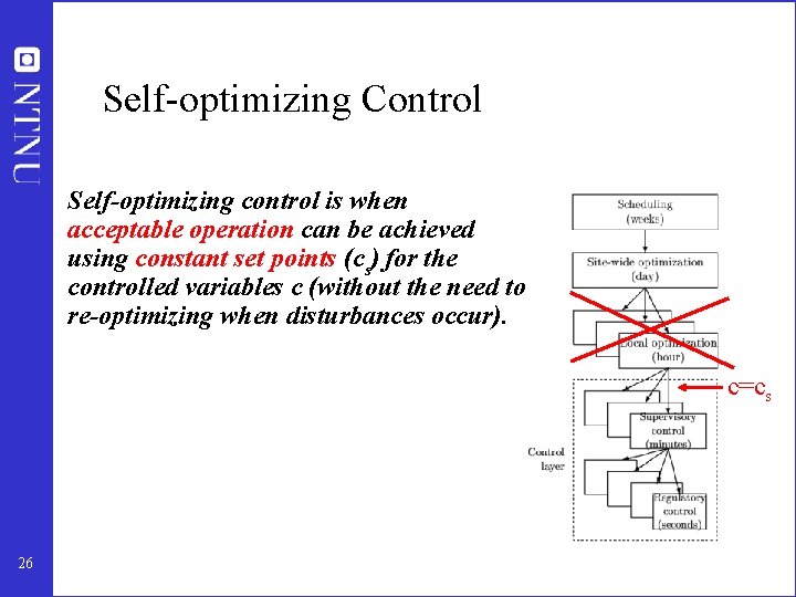
Self-optimizing Control Self-optimizing control is when acceptable operation can be achieved using constant set points (cs) for the controlled variables c (without the need to re-optimizing when disturbances occur). c=cs 26

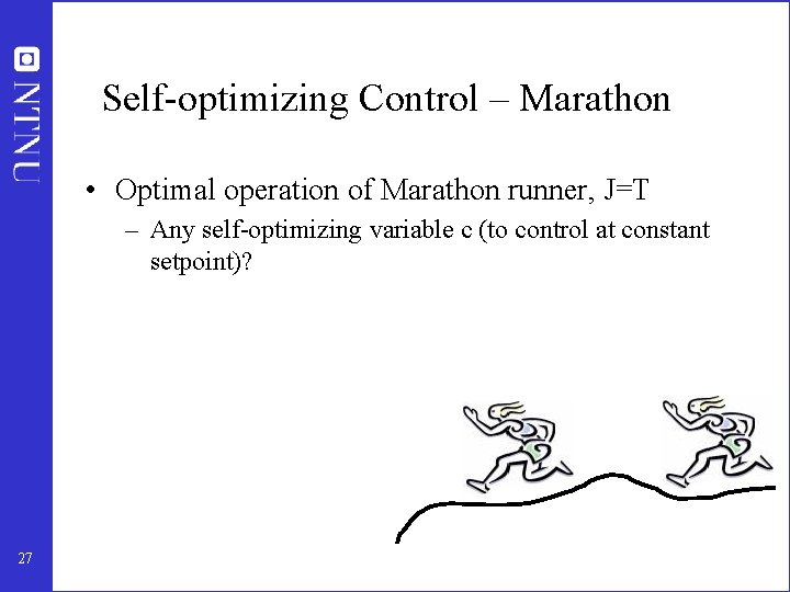
Self-optimizing Control – Marathon • Optimal operation of Marathon runner, J=T – Any self-optimizing variable c (to control at constant setpoint)? 27

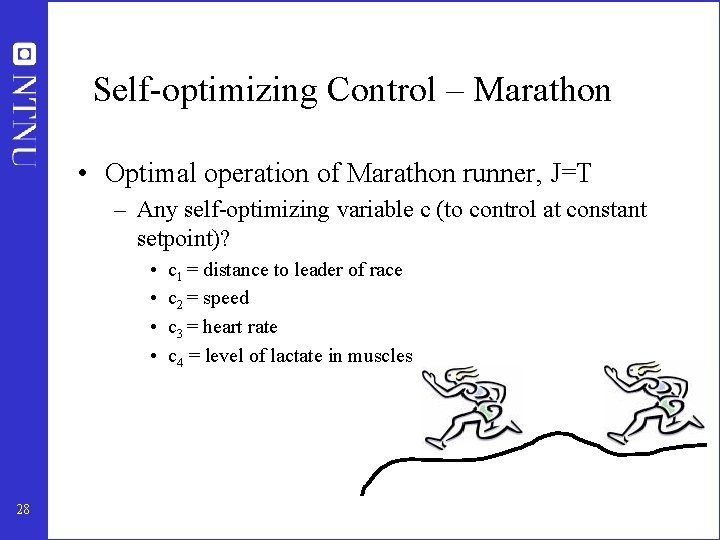
Self-optimizing Control – Marathon • Optimal operation of Marathon runner, J=T – Any self-optimizing variable c (to control at constant setpoint)? • • 28 c 1 = distance to leader of race c 2 = speed c 3 = heart rate c 4 = level of lactate in muscles

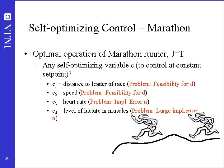
Self-optimizing Control – Marathon • Optimal operation of Marathon runner, J=T – Any self-optimizing variable c (to control at constant setpoint)? • • 29 c 1 = distance to leader of race (Problem: Feasibility for d) c 2 = speed (Problem: Feasibility for d) c 3 = heart rate (Problem: Impl. Error n) c 4 = level of lactate in muscles (Problem: Large impl. error n)

Self-optimizing Control – Sprinter • Optimal operation of Sprinter (100 m), J=T – Active constraint control: • Maximum speed (”no thinking required”) 30

What should we control? Rule: Maximize the scaled gain • Scalar case. Minimum singular value = gain |G| • Maximize scaled gain: |Gs| = |G| / span – |G|: gain from independent variable (u) to candidate controlled variable (c) – span (of c) = optimal variation in c + control error for c 31

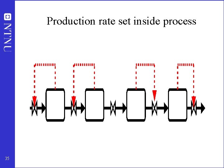
Step 4. Where set production rate? • • 32 Very important! Determines structure of remaining inventory (level) control system Set production rate at (dynamic) bottleneck Link between Top-down and Bottom-up parts

Production rate set at inlet : Inventory control in direction of flow 33

Production rate set at outlet: Inventory control opposite flow 34

Production rate set inside process 35

Where to set the production rate? • Very important decision that determines the structure of the rest of the control system! • May also have important economic implications 36

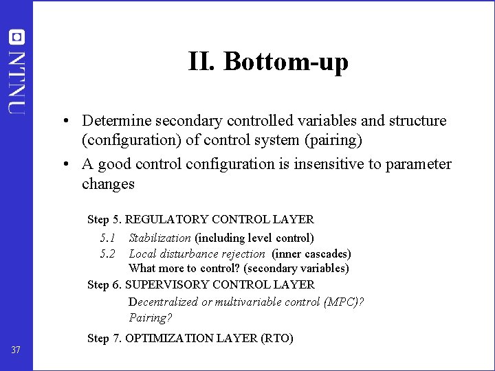
II. Bottom-up • Determine secondary controlled variables and structure (configuration) of control system (pairing) • A good control configuration is insensitive to parameter changes Step 5. REGULATORY CONTROL LAYER 5. 1 Stabilization (including level control) 5. 2 Local disturbance rejection (inner cascades) What more to control? (secondary variables) Step 6. SUPERVISORY CONTROL LAYER Decentralized or multivariable control (MPC)? Pairing? Step 7. OPTIMIZATION LAYER (RTO) 37

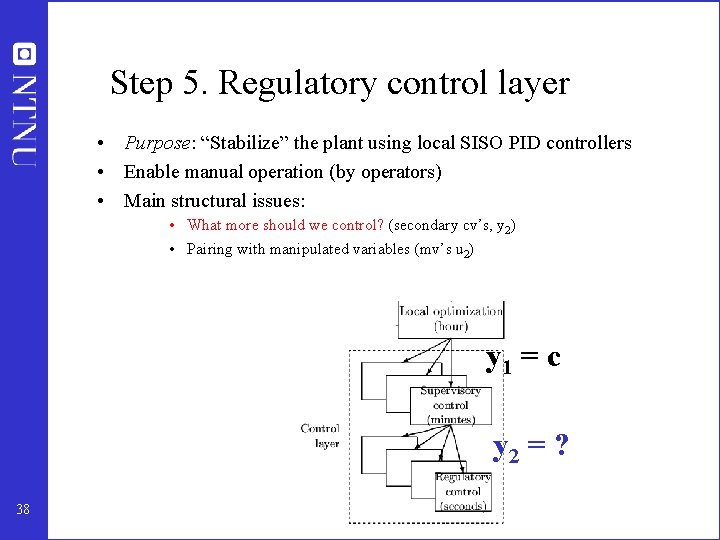
Step 5. Regulatory control layer • Purpose: “Stabilize” the plant using local SISO PID controllers • Enable manual operation (by operators) • Main structural issues: • What more should we control? (secondary cv’s, y 2) • Pairing with manipulated variables (mv’s u 2) y 1 = c y 2 = ? 38

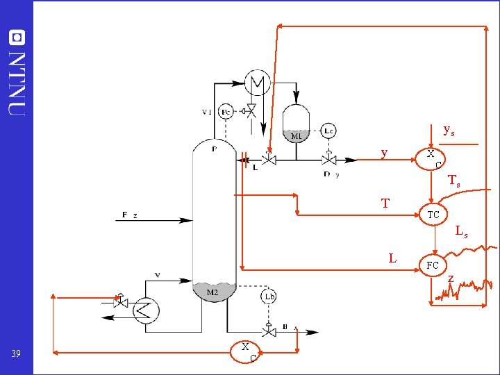
ys y X C Ts T TC Ls L 39 X C FC z

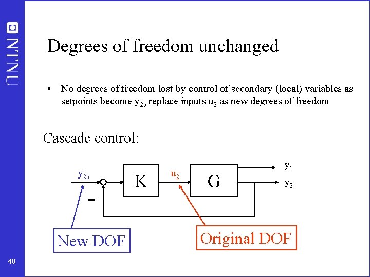
Degrees of freedom unchanged • No degrees of freedom lost by control of secondary (local) variables as setpoints become y 2 s replace inputs u 2 as new degrees of freedom Cascade control: y 2 s New DOF 40 K u 2 G y 1 y 2 Original DOF

What should we control? Rule: Maximize the scaled gain • Scalar case. Minimum singular value = gain |G| • Maximize scaled gain: |Gs| = |G| / span – |G|: gain from independent variable (u) to candidate controlled variable (y) – span (of y) = optimal variation in c + control error for y 41

Step 6. Supervisory control layer • Purpose: Keep primary controlled outputs c=y 1 at optimal setpoints cs • Degrees of freedom: Setpoints y 2 s in reg. control layer • Main structural issue: Decentralized or multivariable? 42

Decentralized control (single-loop controllers) Use for: Noninteracting process and no change in active constraints + Tuning may be done on-line + No or minimal model requirements + Easy to fix and change - Need to determine pairing - Performance loss compared to multivariable control - Complicated logic required for reconfiguration when active constraints move 43

Multivariable control (with explicit constraint handling = MPC) Use for: Interacting process and changes in active constraints + Easy handling of feedforward control + Easy handling of changing constraints • no need for logic • smooth transition - 44 Requires multivariable dynamic model Tuning may be difficult Less transparent “Everything goes down at the same time”

Step 7. Optimization layer (RTO) • Purpose: Identify active constraints and compute optimal setpoints (to be implemented by supervisory control layer) • Main structural issue: Do we need RTO? (or is process selfoptimizing) 45

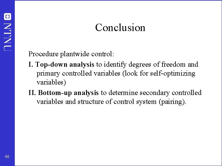
Conclusion Procedure plantwide control: I. Top-down analysis to identify degrees of freedom and primary controlled variables (look for self-optimizing variables) II. Bottom-up analysis to determine secondary controlled variables and structure of control system (pairing). 46

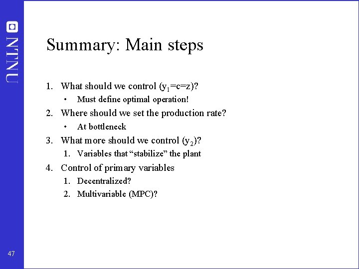
Summary: Main steps 1. What should we control (y 1=c=z)? • Must define optimal operation! 2. Where should we set the production rate? • At bottleneck 3. What more should we control (y 2)? 1. Variables that “stabilize” the plant 4. Control of primary variables 1. Decentralized? 2. Multivariable (MPC)? 47