Plan Embedded Systems New Approaches to building ESW

Plan • Embedded Systems • New Approaches to building ESW – New paradigms: Lava, Handel-C – Examples + “Engineering Returns to Software” – Build a RISC processor in 48 hrs – Advantages of reconfigurable hardware. • Real-time support for ESW © Krithi Ramamritham / Kavi Arya 1

Lava • Not so much a hardware description language • More a style of circuit description • Emphasises connection patterns • Think of Lego © Krithi Ramamritham / Kavi Arya 2

Lava • Mary Sheeran, Koen Classen, & Satnam Singh Chalmers University (Sweden) • Based on earlier work on Mu. FP to describe circuit functionality and layout in single language • Built using functional programming paradigm © Krithi Ramamritham / Kavi Arya 3

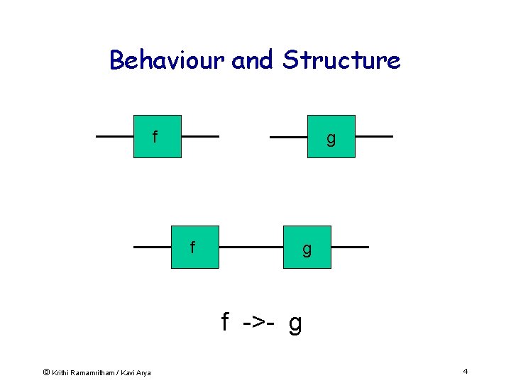
Behaviour and Structure f g f ->- g © Krithi Ramamritham / Kavi Arya 4

Lava Properties • Higher-order functions – Circuits are functions – May be passed as arguments to other functions. – => Easier to produce parameterized circuits than with VHDL. • Functions can return circuits as results – Circuit combinators take circuits as arguments, return circuits as results. – => Powerful glue for composing circuits to form larger systems. • Circuit combinators combine behavior + layout – Combinators lay out circuits in rows, columns, triangles, trees etc. • Performance of circuit – Improved by exploring the layout design space by experimenting with alternative layout combinators. • Examples of circuits produced: – High speed constant coefficient multipliers, finite impulse response filters (1 D and 2 D), adder tree networks and sorting 5 © Krithi Ramamritham / Kavi Arya butterfly networks.

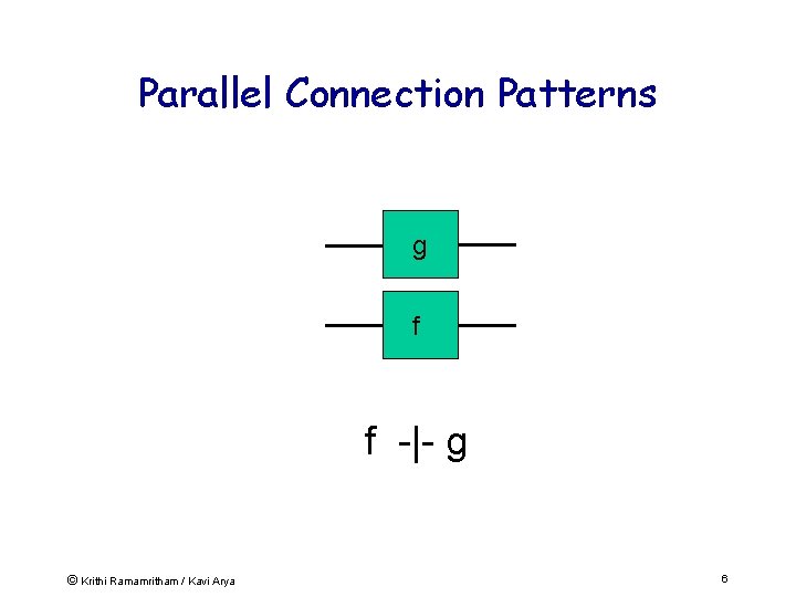
Parallel Connection Patterns g f f -|- g © Krithi Ramamritham / Kavi Arya 6

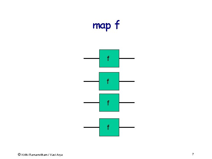
map f f f © Krithi Ramamritham / Kavi Arya 7

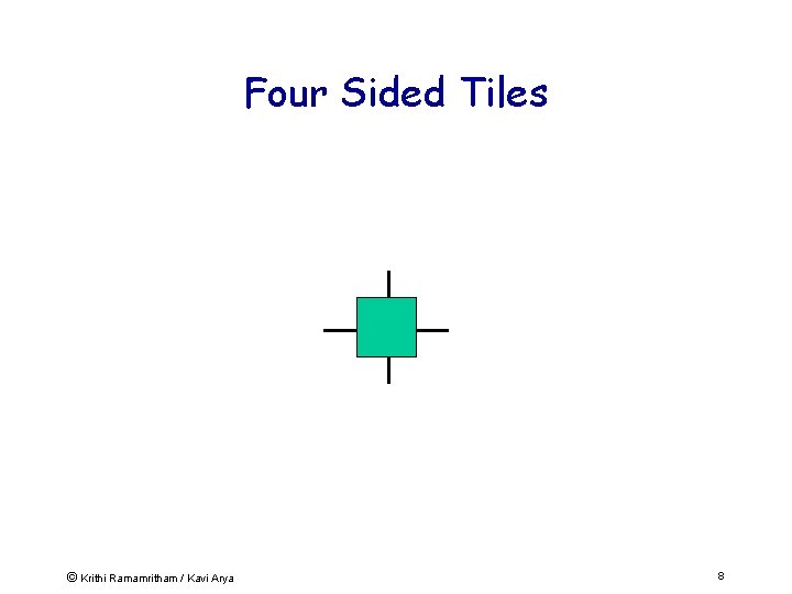
Four Sided Tiles © Krithi Ramamritham / Kavi Arya 8

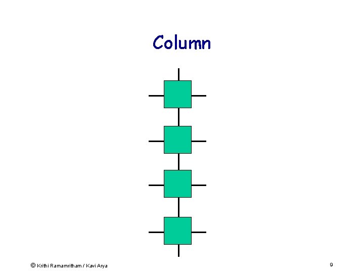
Column © Krithi Ramamritham / Kavi Arya 9

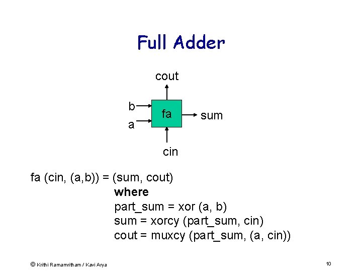
Full Adder cout b a fa sum cin fa (cin, (a, b)) = (sum, cout) where part_sum = xor (a, b) sum = xorcy (part_sum, cin) cout = muxcy (part_sum, (a, cin)) © Krithi Ramamritham / Kavi Arya 10

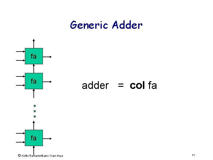
Generic Adder fa fa adder = col fa fa © Krithi Ramamritham / Kavi Arya 11

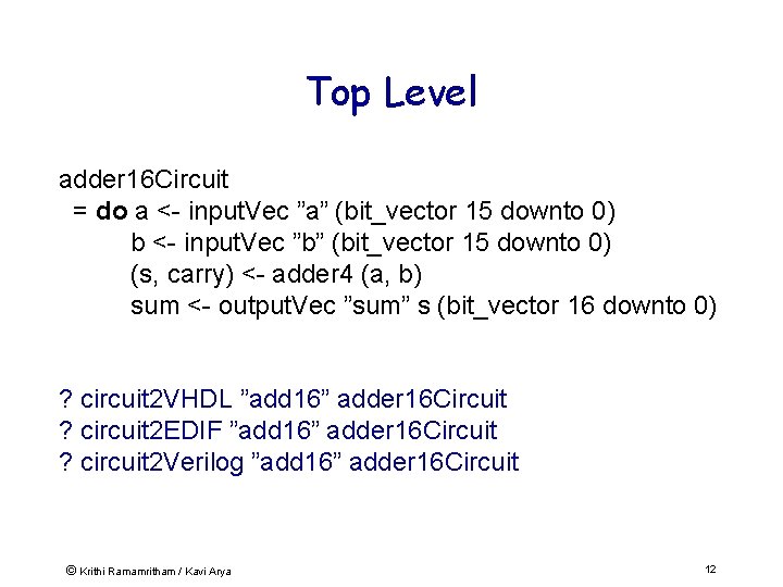
Top Level adder 16 Circuit = do a <- input. Vec ”a” (bit_vector 15 downto 0) b <- input. Vec ”b” (bit_vector 15 downto 0) (s, carry) <- adder 4 (a, b) sum <- output. Vec ”sum” s (bit_vector 16 downto 0) ? circuit 2 VHDL ”add 16” adder 16 Circuit ? circuit 2 EDIF ”add 16” adder 16 Circuit ? circuit 2 Verilog ”add 16” adder 16 Circuit © Krithi Ramamritham / Kavi Arya 12

Xilinx FPGA Implementation • 16 -bit implementation on a XCV 300 FPGA • Vertical layout required to exploit fast carry chain • No need to specify coordinates in HDL code © Krithi Ramamritham / Kavi Arya 13

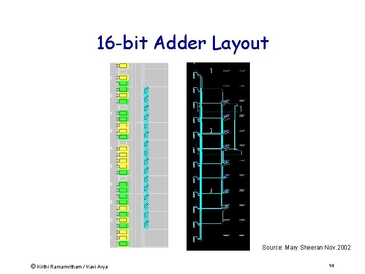
16 -bit Adder Layout Source: Mary Sheeran Nov. 2002 © Krithi Ramamritham / Kavi Arya 14

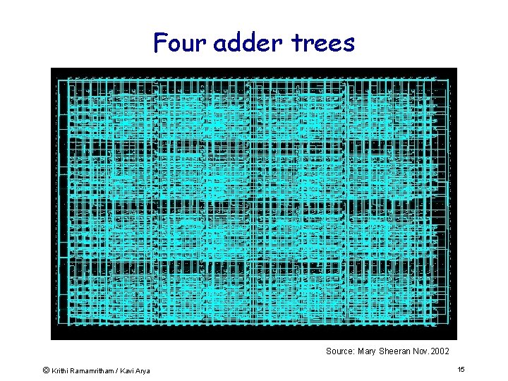
Four adder trees Source: Mary Sheeran Nov. 2002 © Krithi Ramamritham / Kavi Arya 15

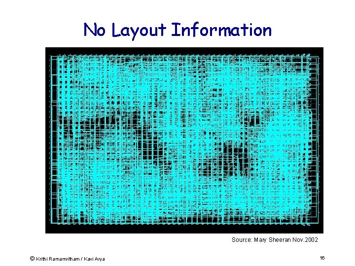
No Layout Information Source: Mary Sheeran Nov. 2002 © Krithi Ramamritham / Kavi Arya 16

Plan • Embedded Systems • New Approaches to building ESW – New paradigms: Lava, Handel-C – Examples + “Engineering Returns to Software” – Build a RISC processor in 48 hrs – Advantages of reconfigurable hardware. • Real-time support for ESW © Krithi Ramamritham / Kavi Arya 17

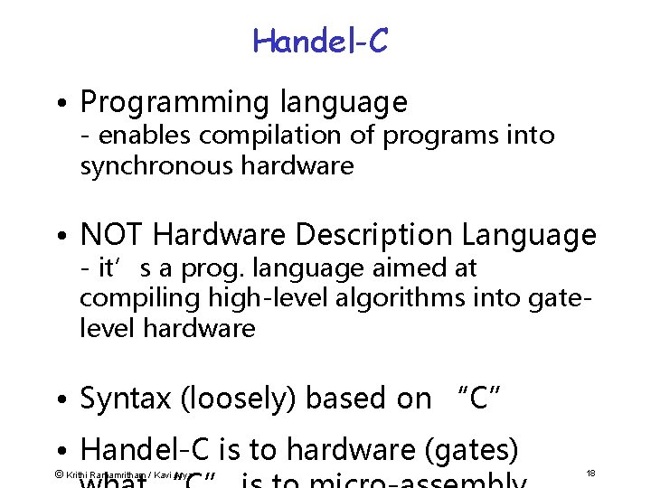
Handel-C • Programming language - enables compilation of programs into synchronous hardware • NOT Hardware Description Language - it’s a prog. language aimed at compiling high-level algorithms into gatelevel hardware • Syntax (loosely) based on “C” • Handel-C is to hardware (gates) © Krithi Ramamritham / Kavi Arya 18

Handel-C (cont. ) • Inventor - Ian Page, Programming Research Group (Oxford University/UK) • Semantics based on Hoare’s Communication Seq. Processes (CSP) model & • Occam: transputer prog. language • Industry heavyweights using tools: Marconi, Ericcson, BAe, Creative Labs, © Krithi Ramamritham / Kavi Arya 19

What this means • Hardware design produced is exactly the hardware specified in source program • No intermediate “interpreting” layer as in assembly language targeting general purpose microprocessor • Logic gates are assembly instructions of Handel-C system © Krithi Ramamritham / Kavi Arya 20

What This Means • True parallelism – not time-shared (interpreted) parallelism of gen. purpose computers • PAR {a; b} – instructions executed in // at same instant of time by 2 sep. pcs of hw • Timing – branches that complete early forced to wait for slowest branch before continuing © Krithi Ramamritham / Kavi Arya 21

Comparison with “C” • Similar: - Programs inherently sequential - Similar control-flow constructs: if-then-else, switch, while, for, etc. • Dissimilar : - No malloc/ dynamic store allocation - No recursion (limited rec. in macros) - No nested procedures - No stdin/stdout - “Void main()” - variable width words - PAR, etc. © Krithi Ramamritham / Kavi Arya 22

Handel-C is based on • ANSI-standard C without external library-functions: – I/O functions: printf(), putc(), scanf(), . . . – File functions: fopen(), fclose(), fprintf(), . . . – String-functions: length(), strcpy(), strcmp(), … – Math-functions: sin(), cos(), sqrt(), … © Krithi Ramamritham / Kavi Arya 23

Supported declarations statements & instructions: • Main program structure • • • Variables Arrays Switch statement FOR Loop Comments Constants Scope & Variable sharing Arithmetic, Relational Logic ops Conditional Execution While loop Do … While Loop © Krithi Ramamritham / Kavi Arya 24

Channel Communication • link!v … link? v – channel input is form of assignment • Provides link between parallel (‘//’) branches – One // branch outputs data onto channel – Other // branch reads data from channel • => Synchronisation © Krithi Ramamritham / Kavi Arya 25

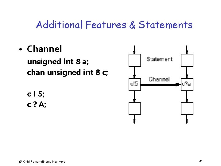
Additional Features & Statements • Channel unsigned int 8 a; chan unsigned int 8 c; c ! 5; c ? A; © Krithi Ramamritham / Kavi Arya 26

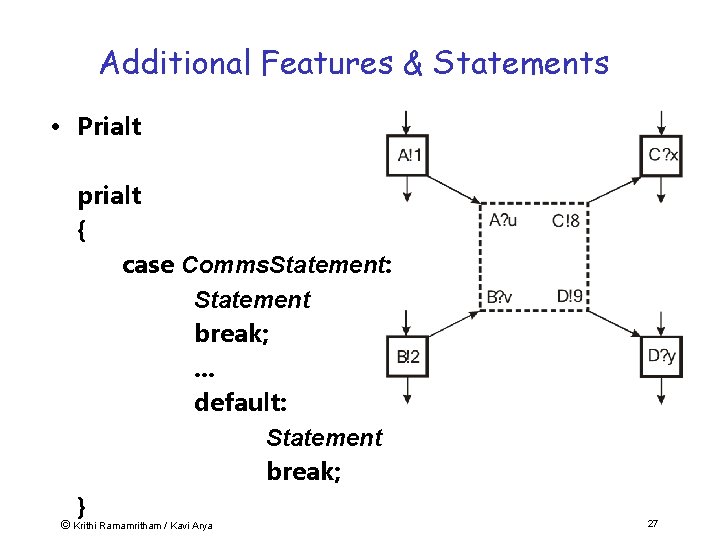
Additional Features & Statements • Prialt prialt { case Comms. Statement: Statement break; . . . default: Statement break; } © Krithi Ramamritham / Kavi Arya 27

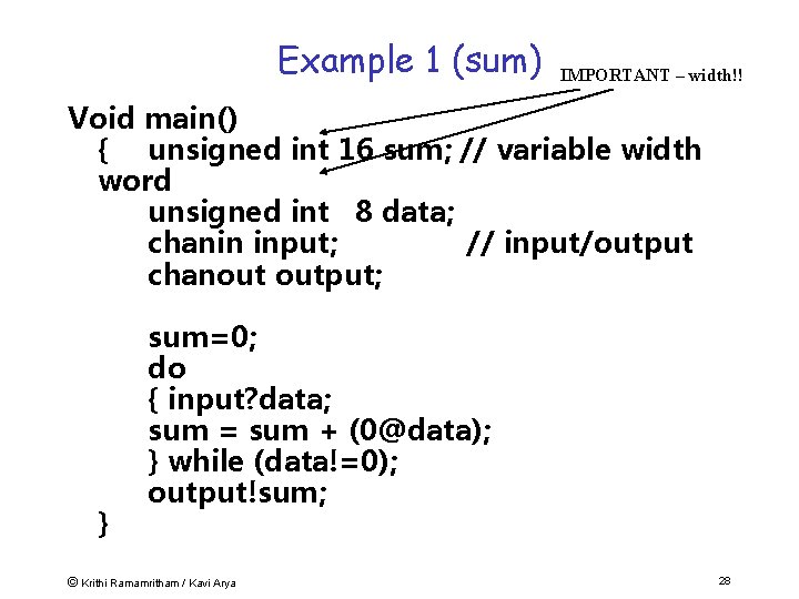
Example 1 (sum) IMPORTANT – width!! Void main() { unsigned int 16 sum; // variable width word unsigned int 8 data; chanin input; // input/output chanout output; } sum=0; do { input? data; sum = sum + (0@data); } while (data!=0); output!sum; © Krithi Ramamritham / Kavi Arya 28

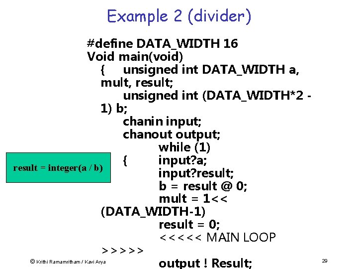
Example 2 (divider) #define DATA_WIDTH 16 Void main(void) { unsigned int DATA_WIDTH a, mult, result; unsigned int (DATA_WIDTH*2 1) b; chanin input; chanout output; while (1) { input? a; result = integer(a / b) input? result; b = result @ 0; mult = 1<< (DATA_WIDTH-1) result = 0; <<<<< MAIN LOOP >>>>> © Krithi Ramamritham / Kavi Arya output ! Result; 29

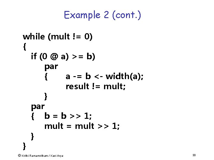
Example 2 (cont. ) while (mult != 0) { if (0 @ a) >= b) par { a -= b <- width(a); result != mult; } par { b = b >> 1; mult = mult >> 1; } } © Krithi Ramamritham / Kavi Arya 30

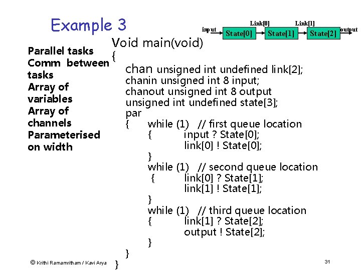
Example 3 input Link[0] State[1] Link[1] Void main(void) Parallel tasks { Comm between chan unsigned int undefined link[2]; tasks Array of variables Array of channels Parameterised on width © Krithi Ramamritham / Kavi Arya } State[2] chanin unsigned int 8 input; chanout unsigned int 8 output unsigned int undefined state[3]; par { while (1) // first queue location { input ? State[0]; link[0] ! State[0]; } while (1) // second queue location { link[0] ? State[1]; link[1] ! State[1]; } while (1) // third queue location { link[1] ? State[2]; output ! State[2]; } } 31 output

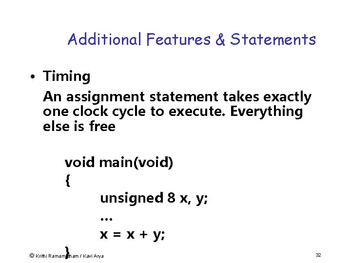
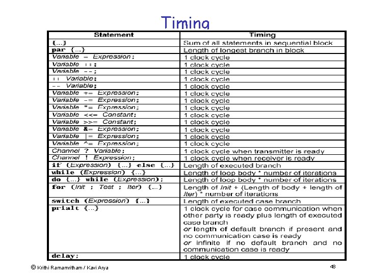
Additional Features & Statements • Timing An assignment statement takes exactly one clock cycle to execute. Everything else is free void main(void) { unsigned 8 x, y; … x = x + y; } © Krithi Ramamritham / Kavi Arya 32

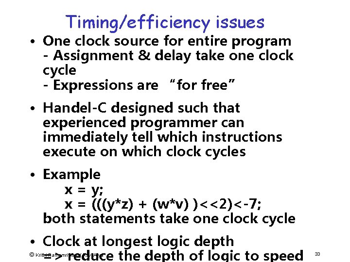
Timing/efficiency issues • One clock source for entire program - Assignment & delay take one clock cycle - Expressions are “for free” • Handel-C designed such that experienced programmer can immediately tell which instructions execute on which clock cycles • Example x = y; x = (((y*z) + (w*v) )<<2)<-7; both statements take one clock cycle • Clock at longest logic depth © => reduce the depth of logic to speed Krithi Ramamritham / Kavi Arya 33

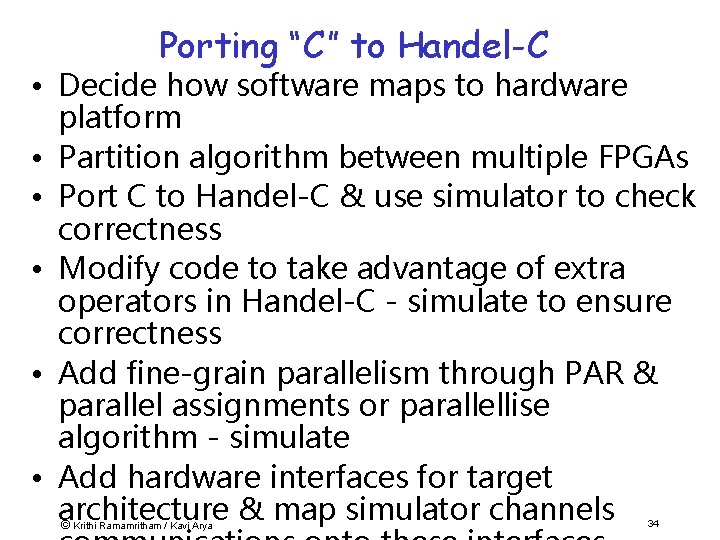
Porting “C” to Handel-C • Decide how software maps to hardware platform • Partition algorithm between multiple FPGAs • Port C to Handel-C & use simulator to check correctness • Modify code to take advantage of extra operators in Handel-C - simulate to ensure correctness • Add fine-grain parallelism through PAR & parallel assignments or parallellise algorithm - simulate • Add hardware interfaces for target architecture & map simulator channels © Krithi Ramamritham / Kavi Arya 34

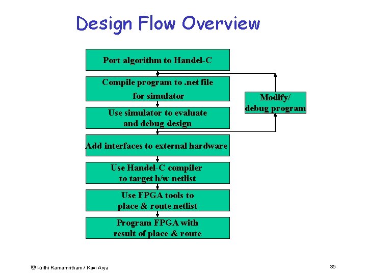
Design Flow Overview Port algorithm to Handel-C Compile program to. net file for simulator Use simulator to evaluate and debug design Modify/ debug program Add interfaces to external hardware Use Handel-C compiler to target h/w netlist Use FPGA tools to place & route netlist Program FPGA with result of place & route © Krithi Ramamritham / Kavi Arya 35

Essence • Software approach allows us to rapidly prototype applications for a given domain • Handel-C provides a seamless approach to derive expressive and fast implementations from the software level • Cost of silicon is falling & shortage of trained engineers & high cost of programmer time © Krithi Ramamritham / Kavi Arya 36

Handel-C Concepts (Recap) • Describes hardware - h/w design produced = h/w in source program • Logic gates are assembly instructions of Handel-C system • Real parallelism – not interpreted • Assignment, delay take 1 clock cycle; Expression evaluation is free • No side-effects I. e. a++ is statement (not expression as in ‘C’) • Variable width words => great performance improvement over software Min. datapath widths => minimal h/w usage © Krithi Ramamritham / Kavi Arya 37

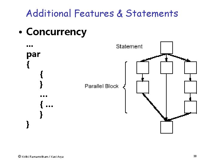
Additional Features & Statements • Concurrency. . . par { { } … {… } } © Krithi Ramamritham / Kavi Arya 38

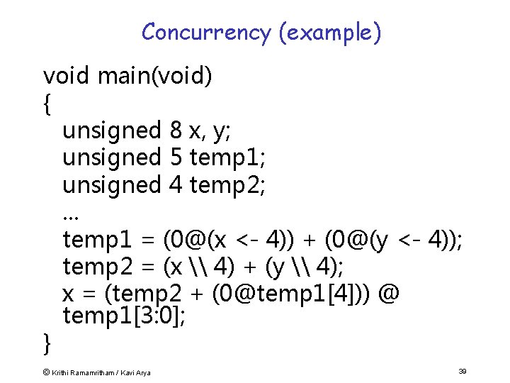
Concurrency (example) void main(void) { unsigned 8 x, y; unsigned 5 temp 1; unsigned 4 temp 2; . . . temp 1 = (0@(x <- 4)) + (0@(y <- 4)); temp 2 = (x \ 4) + (y \ 4); x = (temp 2 + (0@temp 1[4])) @ temp 1[3: 0]; } © Krithi Ramamritham / Kavi Arya 39

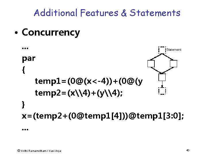
Additional Features & Statements • Concurrency. . . par { temp 1=(0@(x<-4))+(0@(y<-4)); temp 2=(x\4)+(y\4); } x=(temp 2+(0@temp 1[4]))@temp 1[3: 0]; . . . © Krithi Ramamritham / Kavi Arya 40

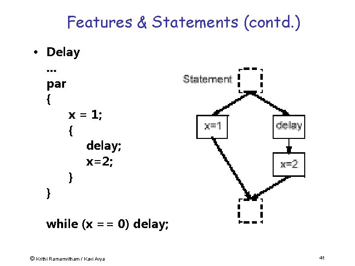
Features & Statements (contd. ) • Delay. . . par { x = 1; { delay; x=2; } } while (x == 0) delay; © Krithi Ramamritham / Kavi Arya 41

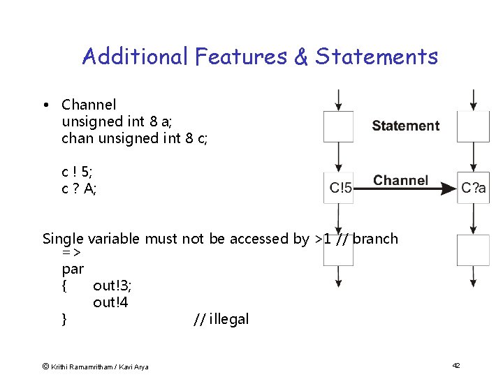
Additional Features & Statements • Channel unsigned int 8 a; chan unsigned int 8 c; c ! 5; c ? A; Single variable must not be accessed by >1 // branch => par { out!3; out!4 } // illegal © Krithi Ramamritham / Kavi Arya 42

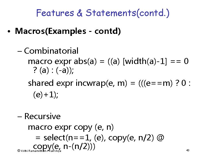
Features & Statements(contd. ) • Macros(Examples - contd) – Combinatorial macro expr abs(a) = ((a) [width(a)-1] == 0 ? (a) : (-a)); shared expr incwrap(e, m) = (((e==m) ? 0 : (e)+1); – Recursive macro expr copy (e, n) = select(n==1, (e), copy(e, n/2) @ copy(e, n-(n/2))) © Krithi Ramamritham / Kavi Arya 43

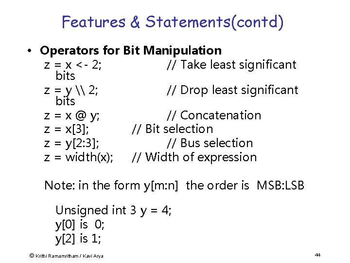
Features & Statements(contd) • Operators for Bit Manipulation z = x <- 2; // Take least significant bits z = y \ 2; // Drop least significant bits z = x @ y; // Concatenation z = x[3]; // Bit selection z = y[2: 3]; // Bus selection z = width(x); // Width of expression Note: in the form y[m: n] the order is MSB: LSB Unsigned int 3 y = 4; y[0] is 0; y[2] is 1; © Krithi Ramamritham / Kavi Arya 44

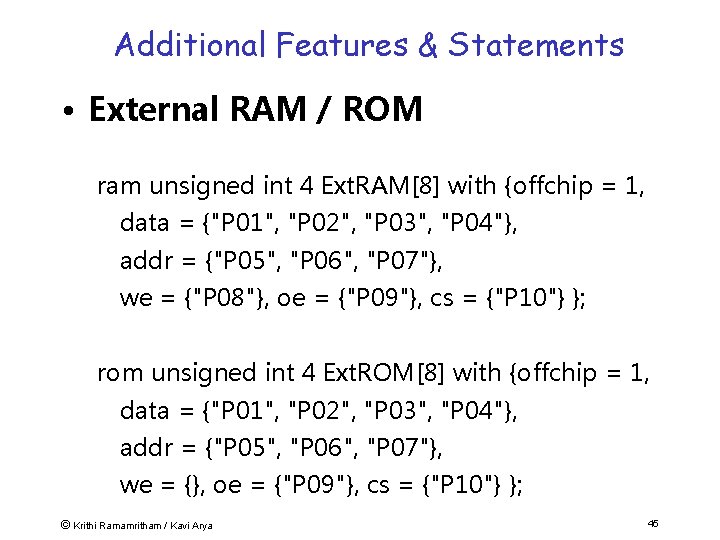
Additional Features & Statements • External RAM / ROM ram unsigned int 4 Ext. RAM[8] with {offchip = 1, data = {"P 01", "P 02", "P 03", "P 04"}, addr = {"P 05", "P 06", "P 07"}, we = {"P 08"}, oe = {"P 09"}, cs = {"P 10"} }; rom unsigned int 4 Ext. ROM[8] with {offchip = 1, data = {"P 01", "P 02", "P 03", "P 04"}, addr = {"P 05", "P 06", "P 07"}, we = {}, oe = {"P 09"}, cs = {"P 10"} }; © Krithi Ramamritham / Kavi Arya 45

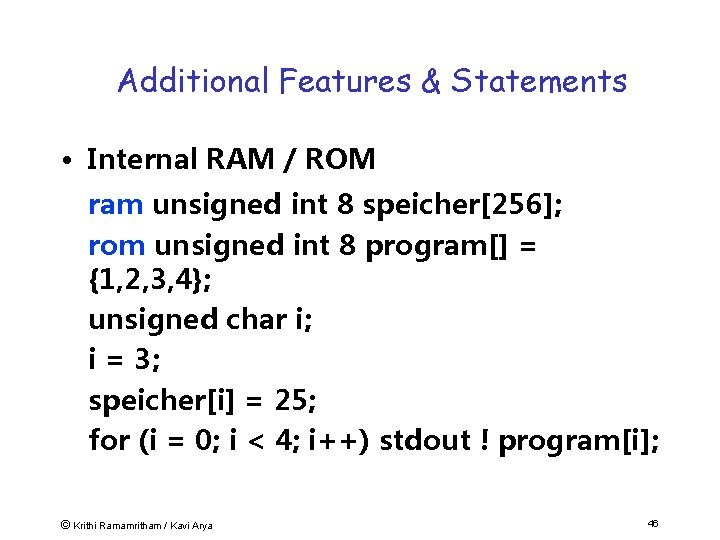
Additional Features & Statements • Internal RAM / ROM ram unsigned int 8 speicher[256]; rom unsigned int 8 program[] = {1, 2, 3, 4}; unsigned char i; i = 3; speicher[i] = 25; for (i = 0; i < 4; i++) stdout ! program[i]; © Krithi Ramamritham / Kavi Arya 46

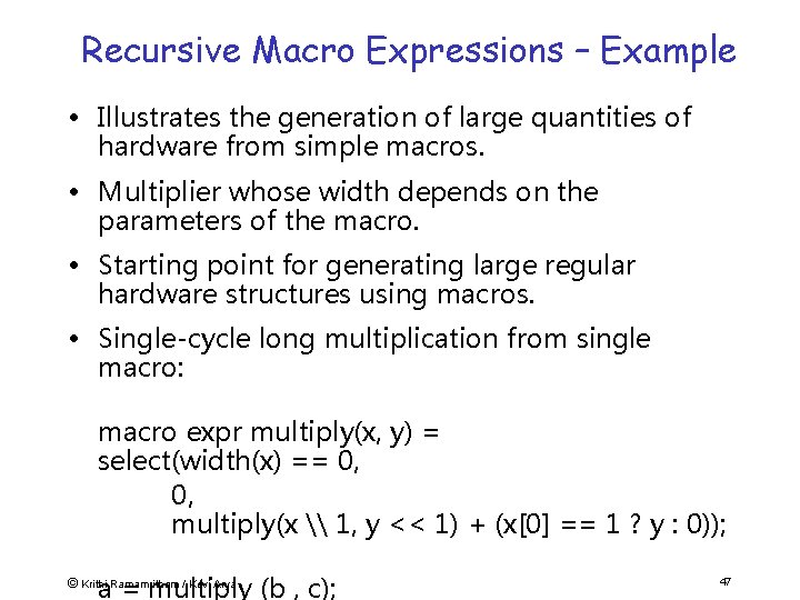
Recursive Macro Expressions – Example • Illustrates the generation of large quantities of hardware from simple macros. • Multiplier whose width depends on the parameters of the macro. • Starting point for generating large regular hardware structures using macros. • Single-cycle long multiplication from single macro: macro expr multiply(x, y) = select(width(x) == 0, 0, multiply(x \ 1, y << 1) + (x[0] == 1 ? y : 0)); a = multiply (b , c); © Krithi Ramamritham / Kavi Arya 47

Timing © Krithi Ramamritham / Kavi Arya 48

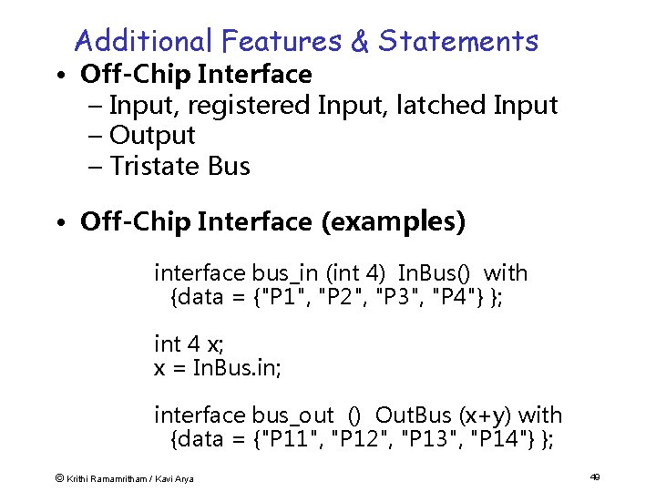
Additional Features & Statements • Off-Chip Interface – Input, registered Input, latched Input – Output – Tristate Bus • Off-Chip Interface (examples) interface bus_in (int 4) In. Bus() with {data = {"P 1", "P 2", "P 3", "P 4"} }; int 4 x; x = In. Bus. in; interface bus_out () Out. Bus (x+y) with {data = {"P 11", "P 12", "P 13", "P 14"} }; © Krithi Ramamritham / Kavi Arya 49

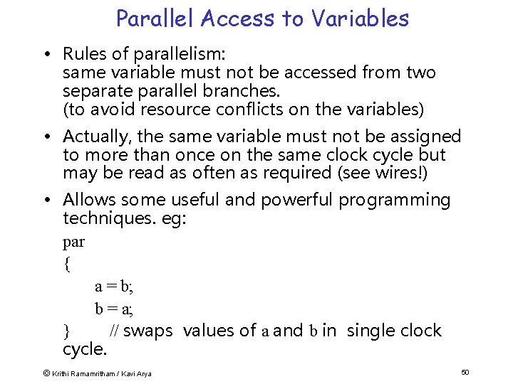
Parallel Access to Variables • Rules of parallelism: same variable must not be accessed from two separate parallel branches. (to avoid resource conflicts on the variables) • Actually, the same variable must not be assigned to more than once on the same clock cycle but may be read as often as required (see wires!) • Allows some useful and powerful programming techniques. eg: par { a = b; b = a; } // swaps values of a and b in single clock cycle. © Krithi Ramamritham / Kavi Arya 50

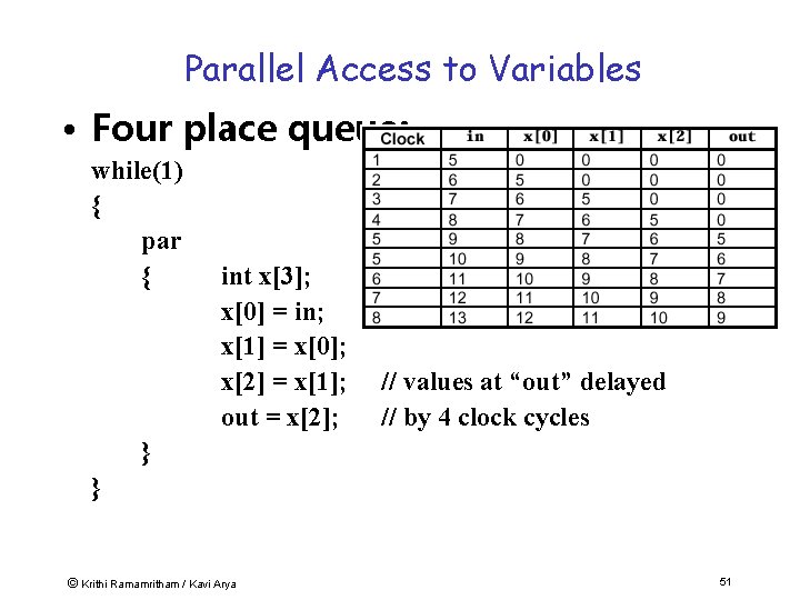
Parallel Access to Variables • Four place queue: while(1) { par { int x[3]; x[0] = in; x[1] = x[0]; x[2] = x[1]; out = x[2]; // values at “out” delayed // by 4 clock cycles } } © Krithi Ramamritham / Kavi Arya 51

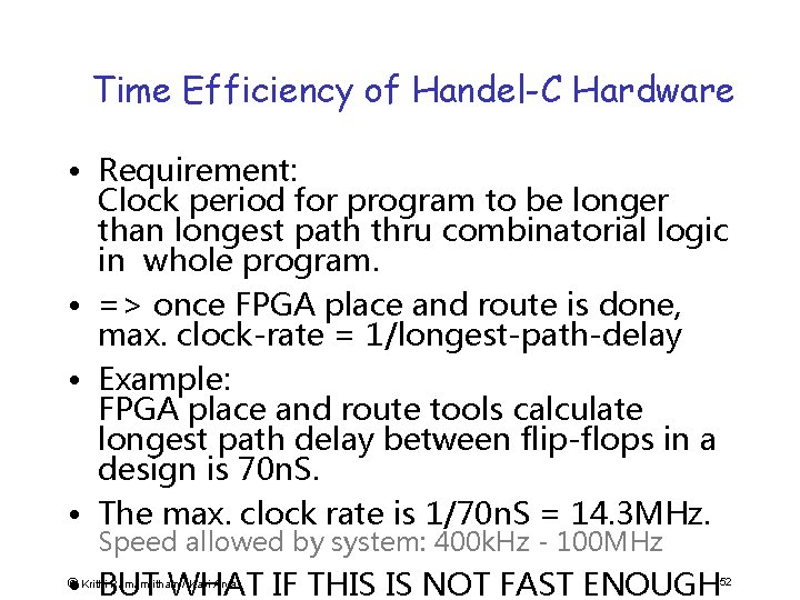
Time Efficiency of Handel-C Hardware • Requirement: Clock period for program to be longer than longest path thru combinatorial logic in whole program. • => once FPGA place and route is done, max. clock-rate = 1/longest-path-delay • Example: FPGA place and route tools calculate longest path delay between flip-flops in a design is 70 n. S. • The max. clock rate is 1/70 n. S = 14. 3 MHz. Speed allowed by system: 400 k. Hz - 100 MHz • BUT WHAT IF THIS IS NOT FAST ENOUGH © Krithi Ramamritham / Kavi Arya 52

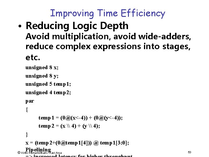
Improving Time Efficiency • Reducing Logic Depth Avoid multiplication, avoid wide-adders, reduce complex expressions into stages, etc. unsigned 8 x; unsigned 8 y; unsigned 5 temp 1; unsigned 4 temp 2; par { temp 1 = (0@(x<-4)) + (0@(y<-4)); temp 2 = (x \ 4) + (y \ 4); } x = (temp 2+(0@temp 1[4])) @ temp 1[3: 0]; Pipelining © Krithi Ramamritham / Kavi Arya 53

Plan • Embedded Systems • New Approaches to building ESW – New paradigms: Lava, Handel-C – Examples (“Engineering Returns to Software” – Build a RISC processor in 48 hrs – Advantages of reconfigurable hardware. • Real-time support for ESW © Krithi Ramamritham / Kavi Arya 56

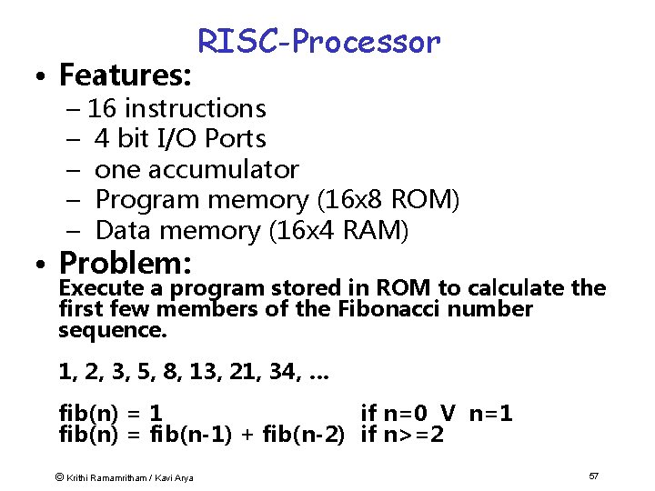
• Features: RISC-Processor – 16 instructions – 4 bit I/O Ports – one accumulator – Program memory (16 x 8 ROM) – Data memory (16 x 4 RAM) • Problem: Execute a program stored in ROM to calculate the first few members of the Fibonacci number sequence. 1, 2, 3, 5, 8, 13, 21, 34, … fib(n) = 1 if n=0 V n=1 fib(n) = fib(n-1) + fib(n-2) if n>=2 © Krithi Ramamritham / Kavi Arya 57

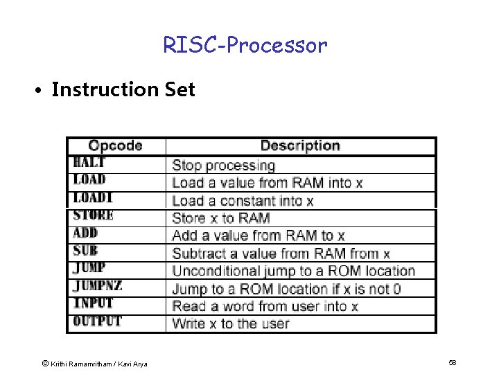
RISC-Processor • Instruction Set © Krithi Ramamritham / Kavi Arya 58

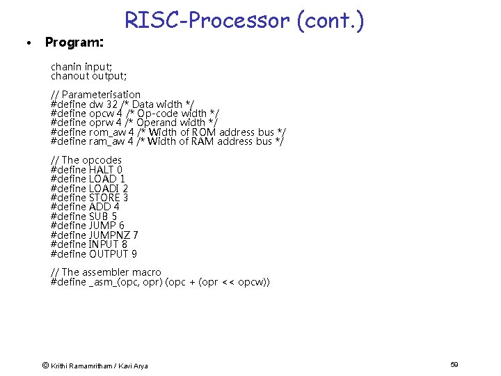
• Program: RISC-Processor (cont. ) chanin input; chanout output; // Parameterisation #define dw 32 /* Data width */ #define opcw 4 /* Op-code width */ #define oprw 4 /* Operand width */ #define rom_aw 4 /* Width of ROM address bus */ #define ram_aw 4 /* Width of RAM address bus */ // The opcodes #define HALT 0 #define LOAD 1 #define LOADI 2 #define STORE 3 #define ADD 4 #define SUB 5 #define JUMP 6 #define JUMPNZ 7 #define INPUT 8 #define OUTPUT 9 // The assembler macro #define _asm_(opc, opr) (opc + (opr << opcw)) © Krithi Ramamritham / Kavi Arya 59

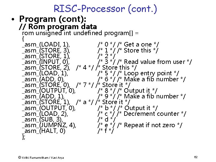
RISC-Processor (cont. ) • Program (cont): // Rom program data rom unsigned int undefined program[] = { _asm_(LOADI, 1), /* 0 */ /* Get a one */ _asm_(STORE, 3), /* 1 */ /* Store this */ _asm_(STORE, 1), /* 2 */ _asm_(INPUT, 0), /* 3 */ /* Read value from user */ _asm_(STORE, 2), /* 4 */ /* Store this */ _asm_(LOAD, 1), /* 5 */ /* Loop entry point */ _asm_(ADD, 0), /* 6 */ /* Make a fib number */ _asm_(STORE, 0), /* 7 */ /* Store it */ _asm_(OUTPUT, 0), /* 8 */ /* Output it */ _asm_(ADD, 1), /* 9 */ /* Make a fib number */ _asm_(STORE, 1), /* a */ /* Store it */ _asm_(OUTPUT, 0), /* b */ /* Output it */ _asm_(LOAD, 2), /* c */ /* Decrement counter */ _asm_(SUB, 3), /* d */ _asm_(JUMPNZ, 4), /* e */ /* Repeat if not zero */ _asm_(HALT, 0) /* f */ }; © Krithi Ramamritham / Kavi Arya 62

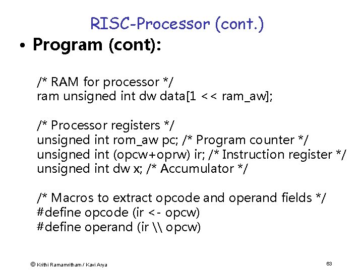
RISC-Processor (cont. ) • Program (cont): /* RAM for processor */ ram unsigned int dw data[1 << ram_aw]; /* Processor registers */ unsigned int rom_aw pc; /* Program counter */ unsigned int (opcw+oprw) ir; /* Instruction register */ unsigned int dw x; /* Accumulator */ /* Macros to extract opcode and operand fields */ #define opcode (ir <- opcw) #define operand (ir \ opcw) © Krithi Ramamritham / Kavi Arya 63

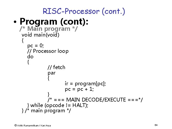
RISC-Processor (cont. ) • Program (cont): /* Main program */ void main(void) { pc = 0; // Processor loop do { // fetch par { ir = program[pc]; pc = pc + 1; } /* === MAIN DECODE/EXECUTE ===*/ } while (opcode != HALT); } /* main program */ © Krithi Ramamritham / Kavi Arya 64

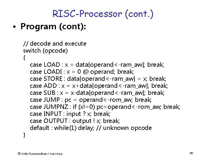
RISC-Processor (cont. ) • Program (cont): // decode and execute switch (opcode) { case LOAD : x = data[operand<-ram_aw]; break; case LOADI : x = 0 @ operand; break; case STORE : data[operand<-ram_aw] = x; break; case ADD : x = x+data[operand<-ram_aw]; break; case SUB : x = x-data[operand<-ram_aw]; break; case JUMP : pc = operand<-rom_aw; break; case JUMPNZ : if (x!=0) pc=operand<-rom_aw; break; case INPUT : input ? x; break; case OUTPUT : output ! x; break; default : while(1) delay; // unknown opcode } © Krithi Ramamritham / Kavi Arya 65

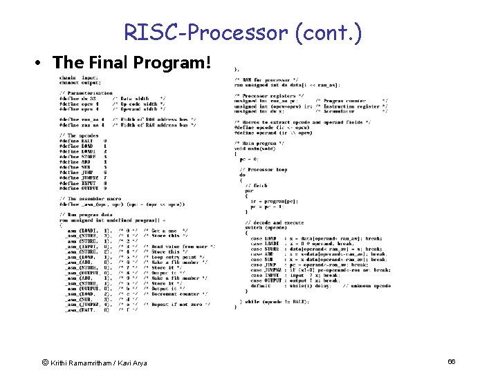
RISC-Processor (cont. ) • The Final Program! © Krithi Ramamritham / Kavi Arya 66

Simulation & debugging • The simulator is integrated into the compiler. • Executing a cycle-based simulation. • Variables are traceable at any clock cycle. • Port interface will be replaced by standard I/O. • Handel-C simulator supports debugging at any clock-cycle. • Highlighting of characteristic Values e. g. Area of any program line. © Krithi Ramamritham / Kavi Arya 67

Some Representative Work • “Customising Graphics Applications: Techniques & Programming Interface” Henry Styles & Wayne Luk, Proceedings of IEEE Symposium on Field Programmable Custom Computing Machines, IEEE Computer Society Press, 2000. • Exploit custom data-formats and datapath widths to optimise graphics operations such as texture mapping & hidden-surface removal. • Discusses techniques for balancing graphics pipeline • Customised architectures captured in Handel -C compiled for Xilinx Virtex FPGAs © Krithi Ramamritham / Kavi Arya 68

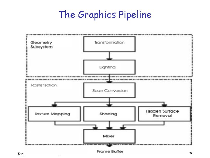
The Graphics Pipeline © Krithi Ramamritham / Kavi Arya 69

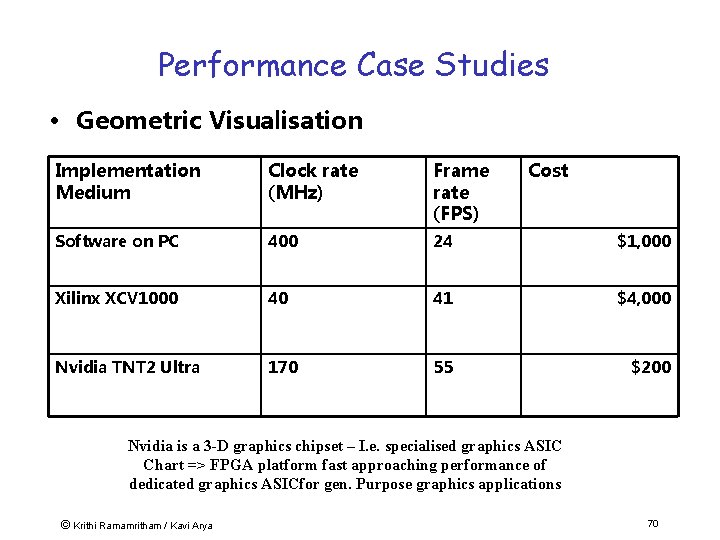
Performance Case Studies • Geometric Visualisation Implementation Medium Clock rate (MHz) Frame rate (FPS) Cost Software on PC 400 24 $1, 000 Xilinx XCV 1000 40 41 $4, 000 Nvidia TNT 2 Ultra 170 55 $200 Nvidia is a 3 -D graphics chipset – I. e. specialised graphics ASIC Chart => FPGA platform fast approaching performance of dedicated graphics ASICfor gen. Purpose graphics applications © Krithi Ramamritham / Kavi Arya 70

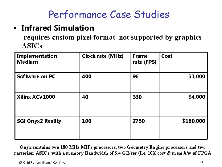
Performance Case Studies • Infrared Simulation requires custom pixel format not supported by graphics ASICs Implementation Medium Clock rate (MHz) Frame Cost rate (FPS) Software on PC 400 96 $1, 000 Xilinx XCV 1000 40 330 $4, 000 SGI Onyx 2 Reality 180 2750 $180, 000 Onyx contains two 180 MHz MIPs processors, two Geometry Engine processors and two rasteriser ASICs, with a memory Bandwidth of 6. 4 GB/sec (I. e. 10 X cost & mem. b/w of FPGA © Krithi Ramamritham / Kavi Arya 71

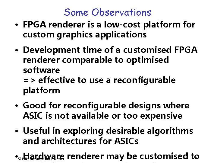
Some Observations • FPGA renderer is a low-cost platform for custom graphics applications • Development time of a customised FPGA renderer comparable to optimised software => effective to use a reconfigurable platform • Good for reconfigurable designs where ASIC is not available or too expensive • Useful in exploring desirable algorithms and architectures for ASICs • © Hardware renderer may be customised to Krithi Ramamritham / Kavi Arya 72

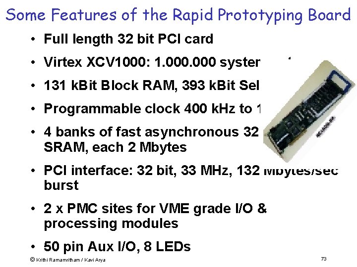
Some Features of the Rapid Prototyping Board • Full length 32 bit PCI card • Virtex XCV 1000: 1. 000 system gates, • 131 k. Bit Block RAM, 393 k. Bit Select. RAM • Programmable clock 400 k. Hz to 100 MHz • 4 banks of fast asynchronous 32 bit wide SRAM, each 2 Mbytes • PCI interface: 32 bit, 33 MHz, 132 Mbytes/sec burst • 2 x PMC sites for VME grade I/O & processing modules • 50 pin Aux I/O, 8 LEDs © Krithi Ramamritham / Kavi Arya 73

Summary • Cost of silicon is falling & Products are getting more complex & Time-to-market shrinking rapidly & shortage of trained engineers & cost of programmer time is major constraint => Software based, high-level approaches to solving problems become increasingly attractive. • New generation of languages let us build systems at high level of abstraction. • High-density FPGAs and So. Cs allow complex designs to be rapidly prototyped => reduce the development cycle of new technology – perhaps even to deploy final product as “soft cores”. • Broader understanding demanded from system designer – need “Renaissance Engineer” with equal understanding of hardware and software. © Krithi Ramamritham / Kavi Arya 74

Plan • Embedded Systems • New Approaches to building ESW • Real-Time Support – Special Characteristics of Real-Time Systems – Real-Time Constraints – Canonical Real-Time Applications – Scheduling in Real-time systems – Operating System Approaches © Krithi Ramamritham / Kavi Arya 75

What is “real” about real-time? computer world e. g. , PC average response for user, at own speed interactive occasionally longer reaction: user annoyed of human life computer controls speed of user “computer time” environment © Krithi Ramamritham / Kavi Arya real world industrial system, airplane events occur in environment reaction too slow: deadline miss reaction: damage, pot. loss computer must follow speed “realof 76

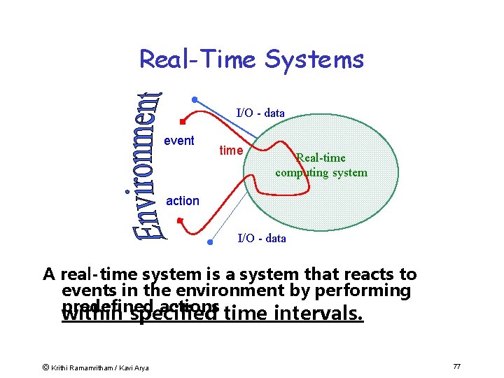
Real-Time Systems I/O - data event time Real-time computing system action I/O - data A real-time system is a system that reacts to events in the environment by performing predefined actions time intervals. within specified © Krithi Ramamritham / Kavi Arya 77

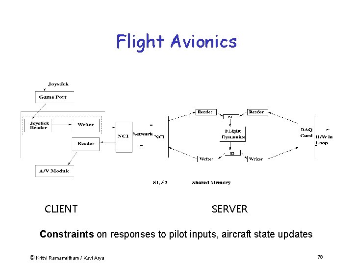
Flight Avionics CLIENT SERVER Constraints on responses to pilot inputs, aircraft state updates © Krithi Ramamritham / Kavi Arya 78

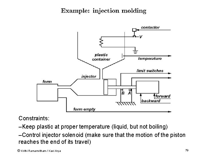
Constraints: –Keep plastic at proper temperature (liquid, but not boiling) –Control injector solenoid (make sure that the motion of the piston reaches the end of its travel) © Krithi Ramamritham / Kavi Arya 79

Real-Time Systems: Properties of Interest • Safety: Nothing bad will happen. • Liveness: Something good will happen. • Timeliness: Things will happen on time -- by their deadlines, periodically, . . © Krithi Ramamritham / Kavi Arya 80

Performance Metrics in Real-Time Systems • Beyond minimizing response times and increasing the throughput: – achieve timeliness. • More precisely, how well can we predict that deadlines will be © Krithi Ramamritham / Kavi Arya 82

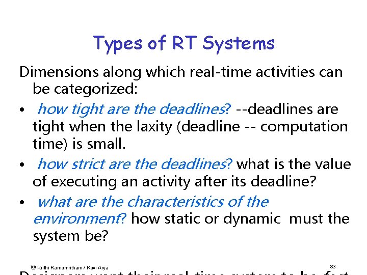
Types of RT Systems Dimensions along which real-time activities can be categorized: • how tight are the deadlines? --deadlines are tight when the laxity (deadline -- computation time) is small. • how strict are the deadlines? what is the value of executing an activity after its deadline? • what are the characteristics of the environment? how static or dynamic must the system be? © Krithi Ramamritham / Kavi Arya 83

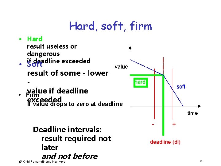
Hard, soft, firm • Hard result useless or dangerous if deadline exceeded • Soft result of some - lower value if deadline • Firm exceeded value hard soft If value drops to zero at deadline time Deadline intervals: result required not later and not before © Krithi Ramamritham / Kavi Arya - + deadline (dl) 84

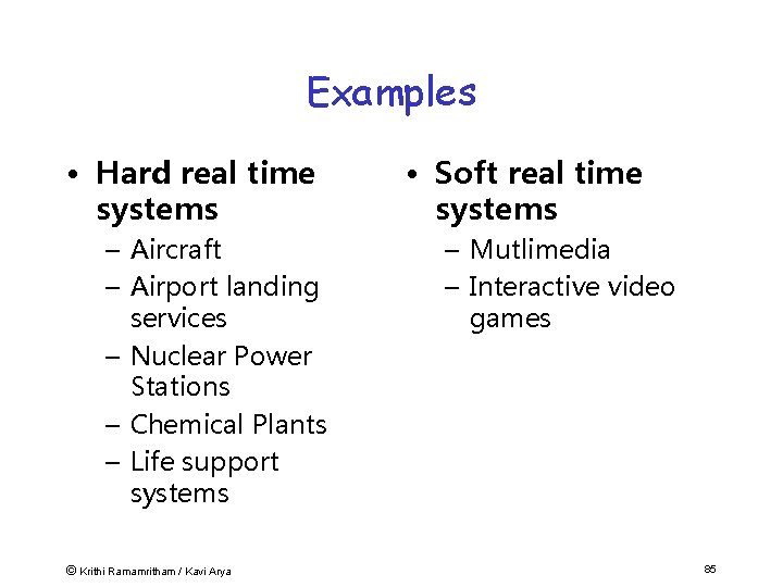
Examples • Hard real time systems – Aircraft – Airport landing services – Nuclear Power Stations – Chemical Plants – Life support systems © Krithi Ramamritham / Kavi Arya • Soft real time systems – Mutlimedia – Interactive video games 85

Real-Time: Items and Terms Task – program, perform service, functionality – requires resources, e. g. , execution time Deadline – specified time for completion of, e. g. , task – time interval or absolute point in time – value of result may depend on completion time © Krithi Ramamritham / Kavi Arya 86

Plan • Special Characteristics of Real-Time Systems • Real-Time Constraints • Canonical Real-Time Applications • Scheduling in Real-time systems • Operating System Approaches © Krithi Ramamritham / Kavi Arya 87

Timing Constraints Real-time means to be in time --how do we know something is “in time”? how do we express that? • Timing constraints are used to specify temporal correctness e. g. , “finish assignment by 2 pm”, “be at station before train departs”. • A system is said to be (temporally) feasible, if it meets all specified timing constraints. • Timing constraints do not come out of © thin air: Krithi Ramamritham / Kavi Arya 88

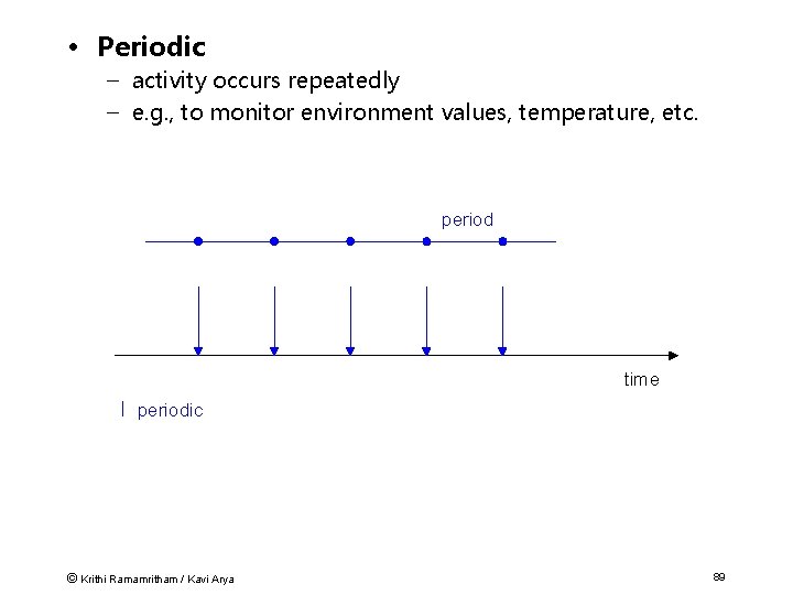
• Periodic – activity occurs repeatedly – e. g. , to monitor environment values, temperature, etc. period time periodic © Krithi Ramamritham / Kavi Arya 89

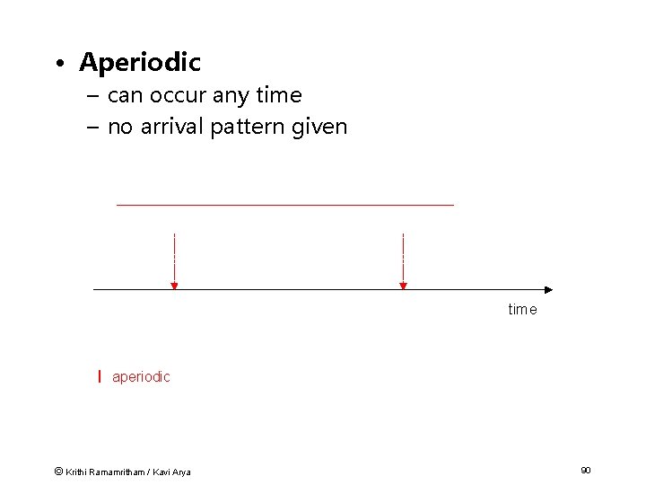
• Aperiodic – can occur any time – no arrival pattern given time aperiodic © Krithi Ramamritham / Kavi Arya 90

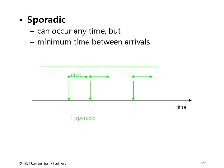
• Sporadic – can occur any time, but – minimum time between arrivals mint time sporadic © Krithi Ramamritham / Kavi Arya 91

Who initiates (triggers) actions? Example: Chemical process – controlled so that temperature stays below danger level – warning is triggered before danger point …… so that cooling can still occur Two possibilities: – action whenever temp raises above warn; event triggered – look every int time intervals; action when temp if measures above warn time triggered © Krithi Ramamritham / Kavi Arya 92

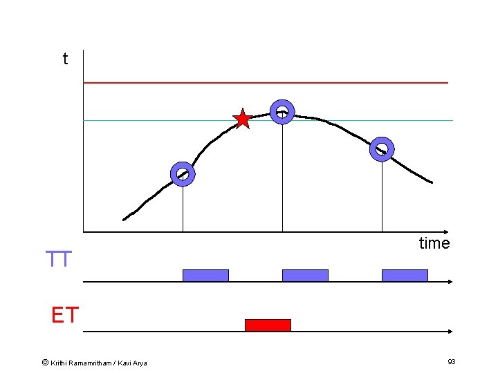
t TT time ET © Krithi Ramamritham / Kavi Arya 93

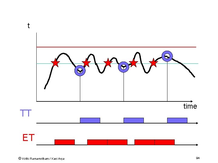
t TT time ET © Krithi Ramamritham / Kavi Arya 94

ET vs TT • Time triggered – Stable number of invocations • Event triggered – Only invoked when needed – High number of invocation and computation demands if value changes frequently © Krithi Ramamritham / Kavi Arya 95

Other Issues to worry about • Meet requirements -- some activities may run only: – after others have completed - precedence constraints – while others are not running - mutual exclusion – within certain times - temporal constraints • Scheduling – planning of activities, such that required timing is kept © Krithi Ramamritham / Kavi Arya 97

Plan • Special Characteristics of Real-Time Systems • Real-Time Constraints • Canonical Real-Time Applications • Scheduling in Real-time systems • Operating System Approaches © Krithi Ramamritham / Kavi Arya 98

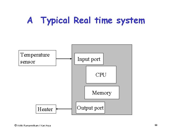
A Typical Real time system Temperature sensor Input port CPU Memory Heater © Krithi Ramamritham / Kavi Arya Output port 99

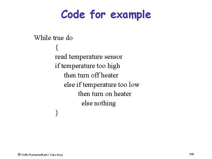
Code for example While true do { read temperature sensor if temperature too high then turn off heater else if temperature too low then turn on heater else nothing } © Krithi Ramamritham / Kavi Arya 100

Comment on code • Code is by Polling device (temperature sensor) • Code is in form of infinite loop • No other tasks can be executed • Suitable for dedicated system or subsystem only © Krithi Ramamritham / Kavi Arya 101

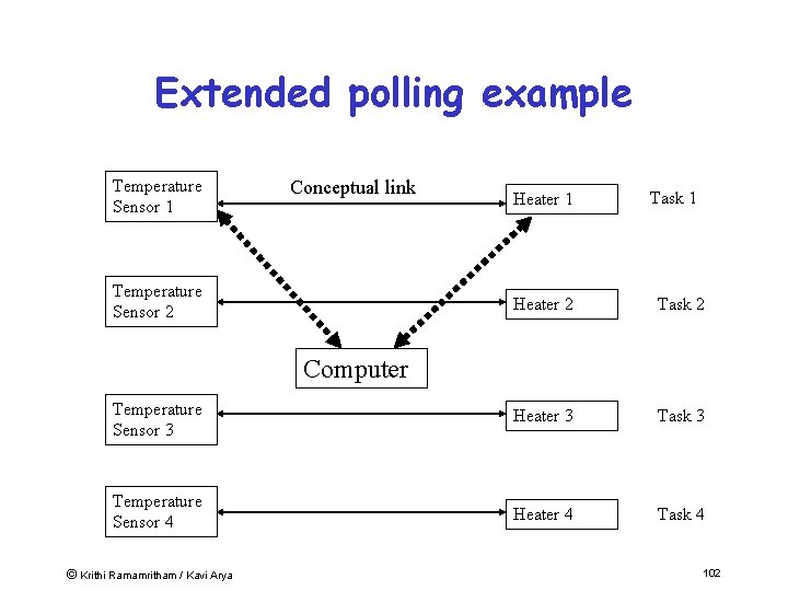
Extended polling example Temperature Sensor 1 Conceptual link Temperature Sensor 2 Heater 1 Task 1 Heater 2 Task 2 Temperature Sensor 3 Heater 3 Task 3 Temperature Sensor 4 Heater 4 Task 4 Computer © Krithi Ramamritham / Kavi Arya 102

Polling • Problems – Arranging task priorities – Round robin is usual within a priority level – Urgent tasks are delayed © Krithi Ramamritham / Kavi Arya 103

Interrupt driven systems • Advantages – Fast – Little delay for high priority tasks • Disadvantages – Programming – Code difficult to debug – Code difficult to maintain © Krithi Ramamritham / Kavi Arya 104

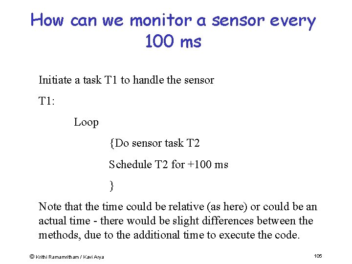
How can we monitor a sensor every 100 ms Initiate a task T 1 to handle the sensor T 1: Loop {Do sensor task T 2 Schedule T 2 for +100 ms } Note that the time could be relative (as here) or could be an actual time - there would be slight differences between the methods, due to the additional time to execute the code. © Krithi Ramamritham / Kavi Arya 105

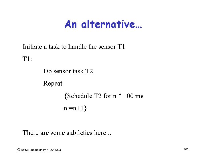
An alternative… Initiate a task to handle the sensor T 1: Do sensor task T 2 Repeat {Schedule T 2 for n * 100 ms n: =n+1} There are some subtleties here. . . © Krithi Ramamritham / Kavi Arya 106

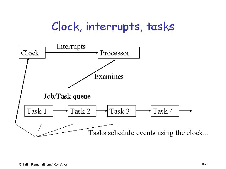
Clock, interrupts, tasks Interrupts Clock Processor Examines Job/Task queue Task 1 Task 2 Task 3 Task 4 Tasks schedule events using the clock. . . © Krithi Ramamritham / Kavi Arya 107

Plan • Special Characteristics of Real-Time Systems • Real-Time Constraints • Canonical Real-Time Applications • Scheduling in Real-time systems • Operating System Approaches © Krithi Ramamritham / Kavi Arya 108

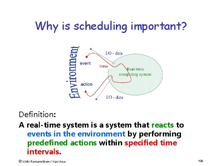
Why is scheduling important? Definition: A real-time system is a system that reacts to events in the environment by performing predefined actions within specified time intervals. © Krithi Ramamritham / Kavi Arya 109

Schedulability analysis a. k. a. feasibility checking: check whether tasks will meet their timing constraints. © Krithi Ramamritham / Kavi Arya 110

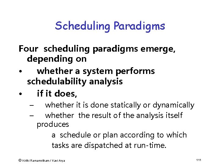
Scheduling Paradigms Four scheduling paradigms emerge, depending on • whether a system performs schedulability analysis • if it does, – – whether it is done statically or dynamically whether the result of the analysis itself produces a schedule or plan according to which tasks are dispatched at run-time. © Krithi Ramamritham / Kavi Arya 111

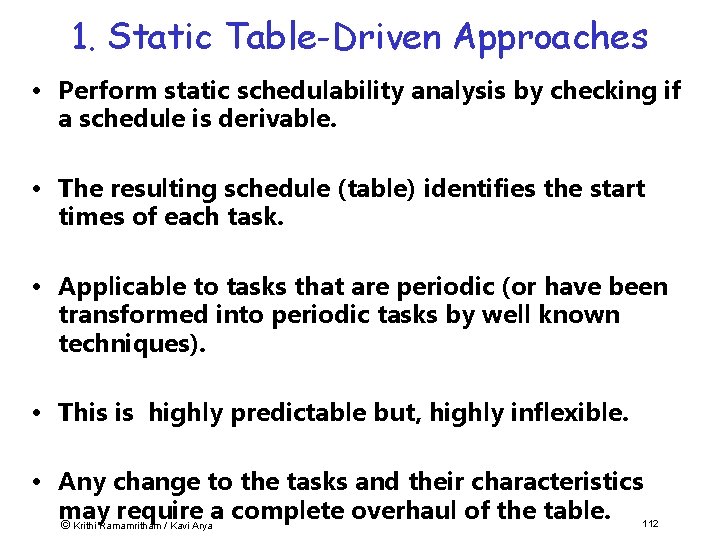
1. Static Table-Driven Approaches • Perform static schedulability analysis by checking if a schedule is derivable. • The resulting schedule (table) identifies the start times of each task. • Applicable to tasks that are periodic (or have been transformed into periodic tasks by well known techniques). • This is highly predictable but, highly inflexible. • Any change to the tasks and their characteristics may require a complete overhaul of the table. 112 © Krithi Ramamritham / Kavi Arya

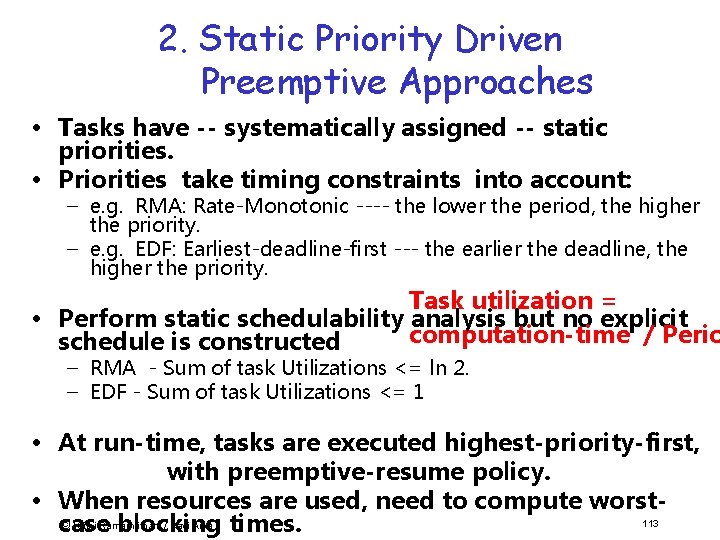
2. Static Priority Driven Preemptive Approaches • Tasks have -- systematically assigned -- static priorities. • Priorities take timing constraints into account: – e. g. RMA: Rate-Monotonic ---- the lower the period, the higher the priority. – e. g. EDF: Earliest-deadline-first --- the earlier the deadline, the higher the priority. Task utilization = • Perform static schedulability analysis but no explicit computation-time / Perio schedule is constructed – RMA - Sum of task Utilizations <= ln 2. – EDF - Sum of task Utilizations <= 1 • At run-time, tasks are executed highest-priority-first, with preemptive-resume policy. • When resources are used, need to compute worst 113 © Krithi Ramamritham / Kavi Arya case blocking times.

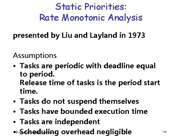
Static Priorities: Rate Monotonic Analysis presented by Liu and Layland in 1973 Assumptions • Tasks are periodic with deadline equal to period. Release time of tasks is the period start time. • Tasks do not suspend themselves • Tasks have bounded execution time • Tasks are independent • © Scheduling overhead negligible Krithi Ramamritham / Kavi Arya 114

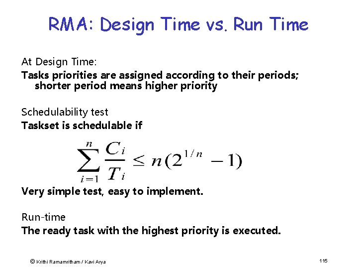
RMA: Design Time vs. Run Time At Design Time: Tasks priorities are assigned according to their periods; shorter period means higher priority Schedulability test Taskset is schedulable if Very simple test, easy to implement. Run-time The ready task with the highest priority is executed. © Krithi Ramamritham / Kavi Arya 115

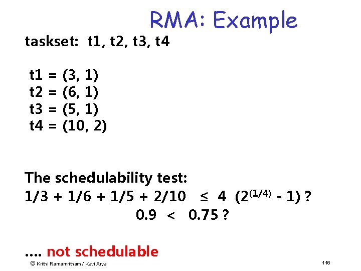
RMA: Example taskset: t 1, t 2, t 3, t 4 t 1 = (3, 1) t 2 = (6, 1) t 3 = (5, 1) t 4 = (10, 2) The schedulability test: 1/3 + 1/6 + 1/5 + 2/10 ≤ 4 (2(1/4) - 1) ? 0. 9 < 0. 75 ? …. not schedulable © Krithi Ramamritham / Kavi Arya 116

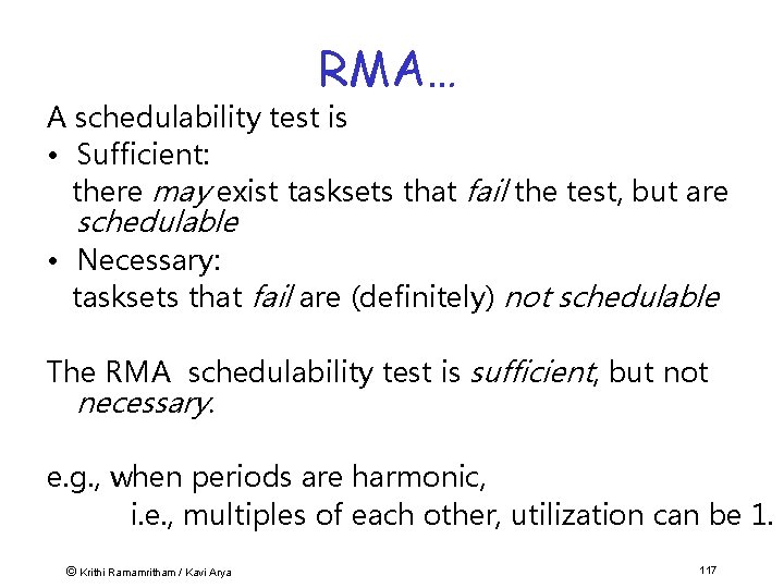
RMA… A schedulability test is • Sufficient: there may exist tasksets that fail the test, but are schedulable • Necessary: tasksets that fail are (definitely) not schedulable The RMA schedulability test is sufficient, but not necessary. e. g. , when periods are harmonic, i. e. , multiples of each other, utilization can be 1. © Krithi Ramamritham / Kavi Arya 117

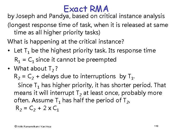
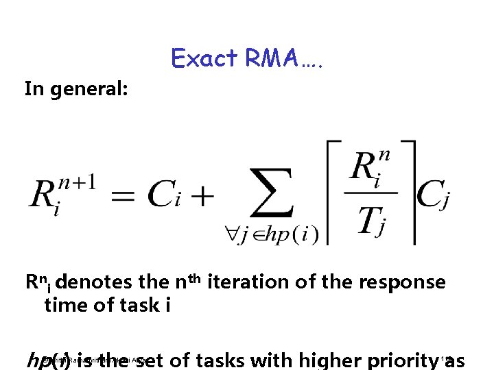
Exact RMA by Joseph and Pandya, based on critical instance analysis (longest response time of task, when it is released at same time as all higher priority tasks) What is happening at the critical instance? • Let T 1 be the highest priority task. Its response time R 1 = C 1 since it cannot be preempted • What about T 2 ? R 2 = C 2 + delays due to interruptions by T 1. Since T 1 has higher priority, it has shorter period. That means it will interrupt T 2 at least once, probably more often. Assume T 1 has half the period of T 2, R 2 = C 2 + 2 x C 1 © Krithi Ramamritham / Kavi Arya 118

Exact RMA…. In general: Rni denotes the nth iteration of the response time of task i hp© (i) is the set of tasks with higher priority as Krithi Ramamritham / Kavi Arya 119

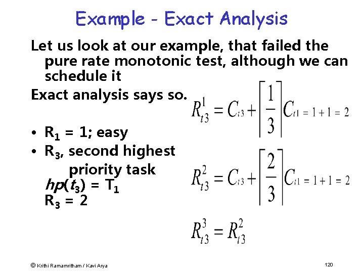
Example - Exact Analysis Let us look at our example, that failed the pure rate monotonic test, although we can schedule it Exact analysis says so. • R 1 = 1; easy • R 3, second highest priority task hp(t 3) = T 1 R 3 = 2 © Krithi Ramamritham / Kavi Arya 120

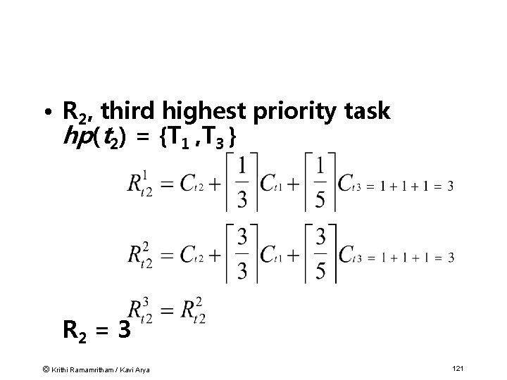
• R 2, third highest priority task hp(t 2) = {T 1 , T 3 } R 2 = 3 © Krithi Ramamritham / Kavi Arya 121

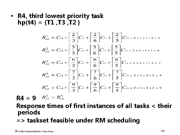
• R 4, third lowest priority task hp(t 4) = {T 1 , T 3 , T 2 } R 4 = 9 Response times of first instances of all tasks < their periods => taskset feasible under RM scheduling © Krithi Ramamritham / Kavi Arya 122

3. Dynamic Planning based Approaches • Feasibility is checked at run-time -- a dynamically arriving task is accepted only if it is feasible to meet its deadline. – Such a task is said to be guaranteed to meet its time constraints • One of the results of the feasibility analysis can be a schedule or plan that determines start times • Has the flexibility of dynamic approaches with some of the predictability of static approaches • If feasibility check is done sufficiently ahead of the deadline, time is available to take alternative actions. © Krithi Ramamritham / Kavi Arya 123

4. Dynamic Best-effort Approaches • The system tries to do its best to meet deadlines. • But since no guarantees are provided, a task may be aborted during its execution. • Until the deadline arrives, or until the task finishes, whichever comes first, one does not know whether a timing constraint will be met. © Krithi Ramamritham / Kavi Arya 124

Cyclic scheduling • Ubiquitous in large-scale dynamic real-time systems • Combination of both table-driven scheduling and priority scheduling. • Tasks are assigned one of a set of harmonic periods. • Within each period, tasks are dispatched according to a table that just lists the order in which the tasks execute. • Slightly more flexible than the table-driven approach • no start times are specified • ©In many actual applications, rather than Krithi Ramamritham / Kavi Arya 125

Plan • Special Characteristics of Real-Time Systems • Real-Time Constraints • Canonical Real-Time Applications • Scheduling in Real-time systems • Operating System Approaches © Krithi Ramamritham / Kavi Arya 126

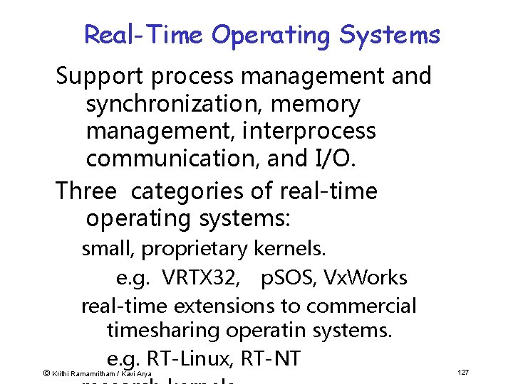
Real-Time Operating Systems Support process management and synchronization, memory management, interprocess communication, and I/O. Three categories of real-time operating systems: small, proprietary kernels. e. g. VRTX 32, p. SOS, Vx. Works real-time extensions to commercial timesharing operatin systems. e. g. RT-Linux, RT-NT © Krithi Ramamritham / Kavi Arya 127

Real-Time Applications Spectrum Hard Soft © Krithi Ramamritham / Kavi Arya Real-Time Operating System General-Purpose Operating System Vx. Works, Lynx, QNX, . . . Intime, Hyper. Kernel, RTX Windows CE Windows NT 128

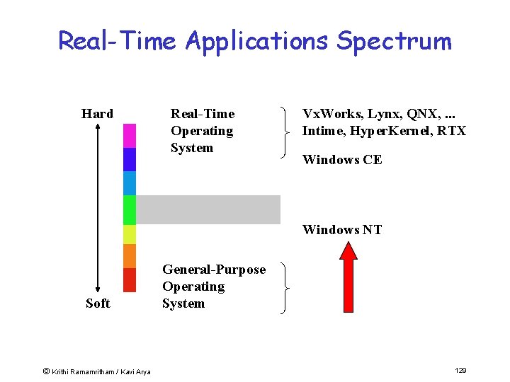
Real-Time Applications Spectrum Hard Real-Time Operating System Vx. Works, Lynx, QNX, . . . Intime, Hyper. Kernel, RTX Windows CE Windows NT Soft © Krithi Ramamritham / Kavi Arya General-Purpose Operating System 129

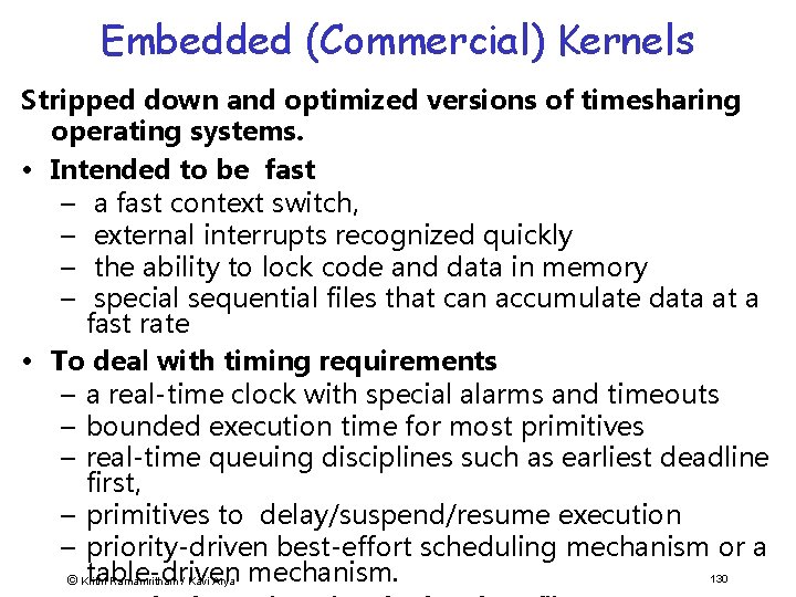
Embedded (Commercial) Kernels Stripped down and optimized versions of timesharing operating systems. • Intended to be fast – a fast context switch, – external interrupts recognized quickly – the ability to lock code and data in memory – special sequential files that can accumulate data at a fast rate • To deal with timing requirements – a real-time clock with special alarms and timeouts – bounded execution time for most primitives – real-time queuing disciplines such as earliest deadline first, – primitives to delay/suspend/resume execution – priority-driven best-effort scheduling mechanism or a table-driven 130 © Krithi Ramamritham / Kavi Arya mechanism.

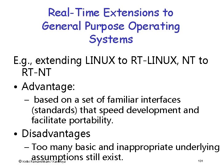
Real-Time Extensions to General Purpose Operating Systems E. g. , extending LINUX to RT-LINUX, NT to RT-NT • Advantage: – based on a set of familiar interfaces (standards) that speed development and facilitate portability. • Disadvantages – Too many basic and inappropriate underlying assumptions still exist. © Krithi Ramamritham / Kavi Arya 131

Using General Purpose Operating Systems • GPOS offer some capabilities useful for real-time system builders • RT applications can obtain leverage from existing development tools and applications • Some GPOSs accepted as de-facto © Krithi Ramamritham / Kavi Arya 132

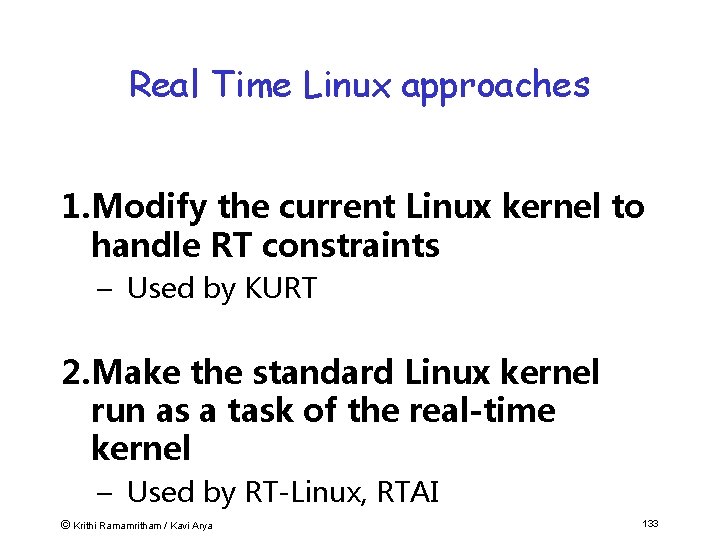
Real Time Linux approaches 1. Modify the current Linux kernel to handle RT constraints – Used by KURT 2. Make the standard Linux kernel run as a task of the real-time kernel – Used by RT-Linux, RTAI © Krithi Ramamritham / Kavi Arya 133

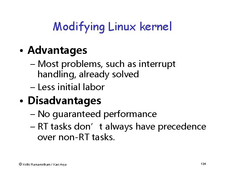
Modifying Linux kernel • Advantages – Most problems, such as interrupt handling, already solved – Less initial labor • Disadvantages – No guaranteed performance – RT tasks don’t always have precedence over non-RT tasks. © Krithi Ramamritham / Kavi Arya 134

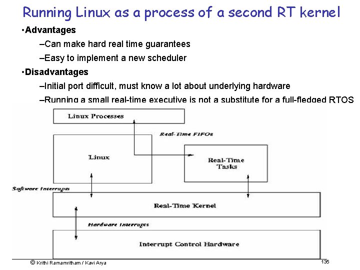
Running Linux as a process of a second RT kernel • Advantages –Can make hard real time guarantees –Easy to implement a new scheduler • Disadvantages –Initial port difficult, must know a lot about underlying hardware –Running a small real-time executive is not a substitute for a full-fledged RTOS © Krithi Ramamritham / Kavi Arya 135

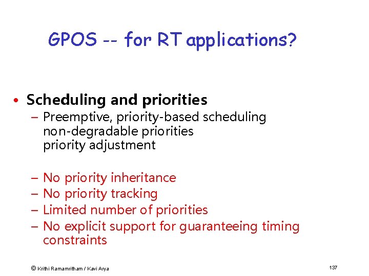
GPOS -- for RT applications? • Scheduling and priorities – Preemptive, priority-based scheduling non-degradable priorities priority adjustment – – No priority inheritance No priority tracking Limited number of priorities No explicit support for guaranteeing timing constraints © Krithi Ramamritham / Kavi Arya 137

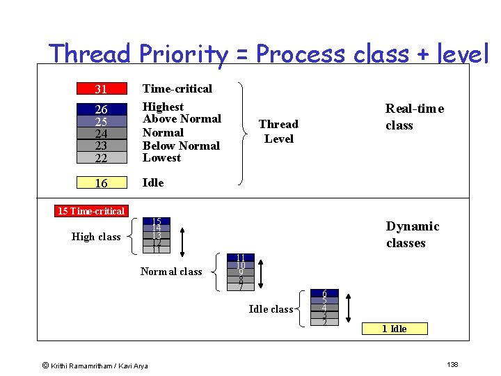
Thread Priority = Process class + level 26 25 24 23 22 Time-critical Highest Above Normal Below Normal Lowest 16 Idle 31 15 Time-critical 15 14 13 12 11 High class Normal class Thread Level Dynamic classes 11 10 9 8 7 Idle class © Krithi Ramamritham / Kavi Arya Real-time class 6 5 4 3 2 1 Idle 138

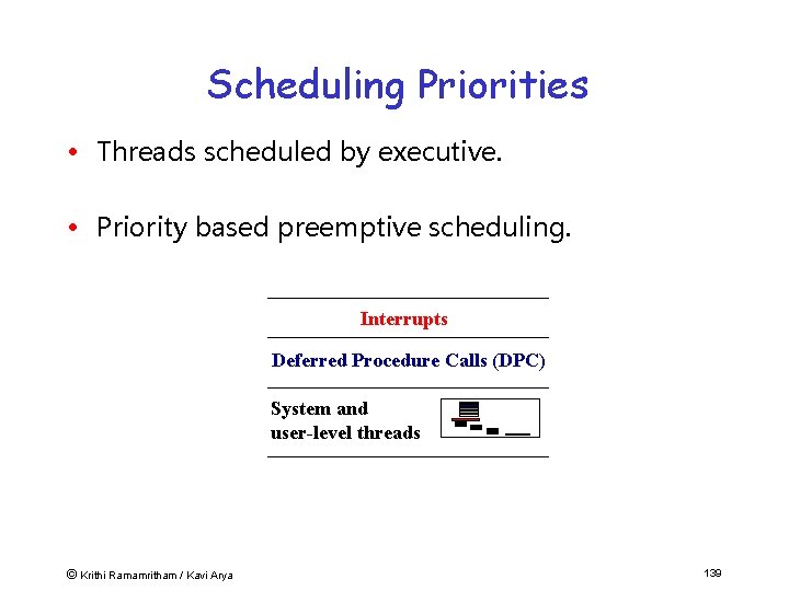
Scheduling Priorities • Threads scheduled by executive. • Priority based preemptive scheduling. Interrupts Deferred Procedure Calls (DPC) System and user-level threads © Krithi Ramamritham / Kavi Arya 139

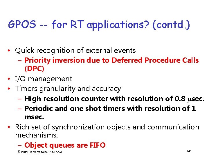
GPOS -- for RT applications? (contd. ) • Quick recognition of external events – Priority inversion due to Deferred Procedure Calls (DPC) • I/O management • Timers granularity and accuracy – High resolution counter with resolution of 0. 8 sec. – Periodic and one shot timers with resolution of 1 msec. • Rich set of synchronization objects and communication mechanisms. – Object queues are FIFO © Krithi Ramamritham / Kavi Arya 140

Research Operating Systems • MARS – static scheduling • ARTS – static priority scheduling • Spring –dynamic guarantees © Krithi Ramamritham / Kavi Arya 141

MARS -- TU, Vienna (Kopetz) Offers support for controlling a distributed application based entirely on time events (rather than asynchronous events) from the environment. • A priori static analysis to demonstrate that all the timing requirements are met. • Uses flow control} on the maximum number of events that the system handles. • Based on the time driven model -- assume everything is periodic. • Static table-driven scheduling approach • A hardware based clock synchronization algorithm • A TDMA-like protocol to guarantee timely 142 © Krithi Ramamritham / Kavi Arya

ARTS -- CMU (Tokuda, et al) • The ARTS kernel provides a distributed realtime computing environment. • Works in conjunction with the static priority driven preemptive scheduling paradigm. • Kernel is tied to various tools that a priori analyze schedulability. • The kernel supports the notion of real-time objects and real-time threads. • Each real-time object is time encapsulated -a time fence mechanism: The time fence provides a run time check that ensures that the slack time is greater than the worst case © Krithi Ramamritham / Kavi Arya 143

SPRING – Umass. (Ramamritham & Stankovic) • Real-time support for multiprocessors and distributed sys • Strives for a more flexible combination of offline and on-line techniques – Safety-critical tasks are dealt with via static tabledriven scheduling. – Dynamic planning based scheduling of tasks that arrive dynamically. • Takes tasks' time and resource constraints into account and avoids the need to a priori compute worst case blocking times • Reflective kernel retains a significant amount of© application semantics at run time – Krithi Ramamritham / Kavi Arya 144

Polis: Synthesizing OSs • Given a FSM description of a RT application • Each FSM becomes a task • Signals, Interrupts, and polling • Tasks with waiting inputs handled in FIFS order (priority order – TB done) • Some interrupts can be made to directly execute the corresponding task • Needed OS execute synthesized based © Krithi Ramamritham / Kavi Arya 145

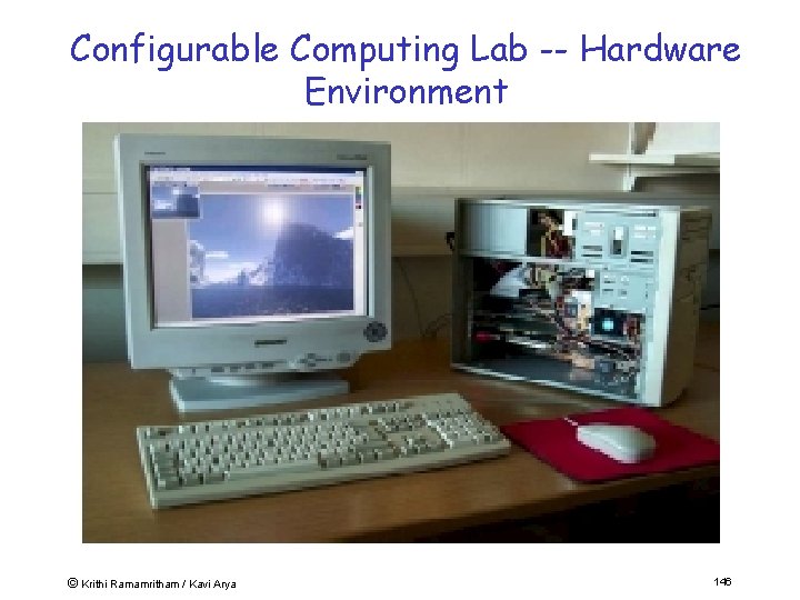
Configurable Computing Lab -- Hardware Environment © Krithi Ramamritham / Kavi Arya 146

IIT-KRe. SIT Reconfigurable Computing Lab Projects (2003) • Network packet-processing - Packet Classifier (a la Stiliades/ Laxman) • Wireless Protocol – 802. 11 interface card • Video codec - MPEG-4 with encryption • Encryption (IDEA, etc. ) • Real-time reactive control systems - Inertial Navigation System (ILS) - Flight simulation - Scheduling co-processor • Satellite Error Correcting codec © Krithi Ramamritham / Kavi Arya 147

References This tutorial is a short version of a sememster-long course. Visit http: //www. it. iitb. ac. in/~it 606 for all the material from that course • Jack Ganssle, "The Art of Designing Embedded Systems", Newnes, 1999. • David Simon, "An Embedded Software Primer", Addison Wesley, 2000. • C. M. Krishna and Kang G. Shin, "RTS: Real-Time Systems", Mc. Graw-Hill, 1997, ISBN 0 -07 -057043. • Frank Vahid, Tony Givargis, "Embedded System Design: A Unified Hardware/ Software Introduction", John Wiley & Sons Inc. , 2002. © Krithi Ramamritham / Kavi Arya 148

References… • K. Ramamritham and J. A. Stankovic, Scheduling Algorithms and Operating Systems Support for Real-Time Systems, invited paper, Proceedings of the IEEE, Jan 1994, pp. 55 -67. • Sundeep Kapila, K. Ramamritham, Sudhakar, Distributed Real-Time Embedded Applications using Off-the-Shelf Components? Experiences Building a Flight Simulator, IEEE/IEE Real-Time Embedded Systems Workshop (held in conjunction with the IEEE Real-Time Systems Symposium), December 2001. • Real-Time Linux, http: //www. fsmlabs. com/articles/archive/usenix. pdf • Handel-C material based on "Handel-C Language Reference Manual", Celoxica Ltd. 149 © Krithi Ramamritham / Kavi Arya

References… • David Harel, Hagi Lachover, Ammon Naamad, Amir Pnueli, Michal Politi, Rivi Sherman, Aharon Shtull-Trauring, and Mark Trakhtenbrot, Statemate: A working Environment for the Development of Complex Reactive Systems, IEEE Transactions on Software Engineering, Vol 16 No. 4, April 1999. • Ptolemy Project, http: //ptolemy. eecs. berkeley. edu/. • S. Ramesh and P. Bhaduri, Validation of Pipelined processors using Esterel Tools: A Case study, Proc. of Computer Aided Verification, LNCS Vol. 1633, 1999. (pdf version). © Krithi Ramamritham / Kavi Arya 150

Summary • • What are Embedded Systems? What is Embedded software? New Approaches to building ESW Real-time support for ESW © Krithi Ramamritham / Kavi Arya 151