PIVOT TABLES IN EXCEL WHY PIVOT TABLES When

PIVOT TABLES IN EXCEL

WHY PIVOT TABLES? • When you have a lot of data, it can sometimes be difficult to analyze all of the information in your worksheet. Pivot. Tables can help make your worksheets more manageable by summarizing your data and allowing you to manipulate it in different ways.

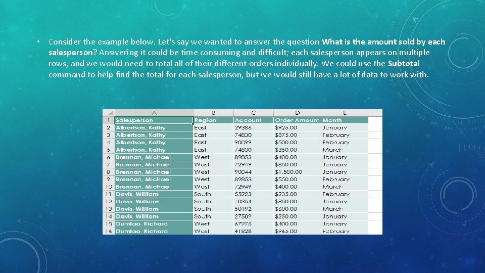
• Consider the example below. Let's say we wanted to answer the question What is the amount sold by each salesperson? Answering it could be time consuming and difficult; each salesperson appears on multiple rows, and we would need to total all of their different orders individually. We could use the Subtotal command to help find the total for each salesperson, but we would still have a lot of data to work with.

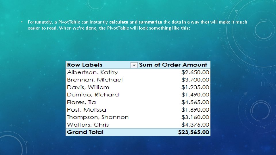
• Fortunately, a Pivot. Table can instantly calculate and summarize the data in a way that will make it much easier to read. When we're done, the Pivot. Table will look something like this:

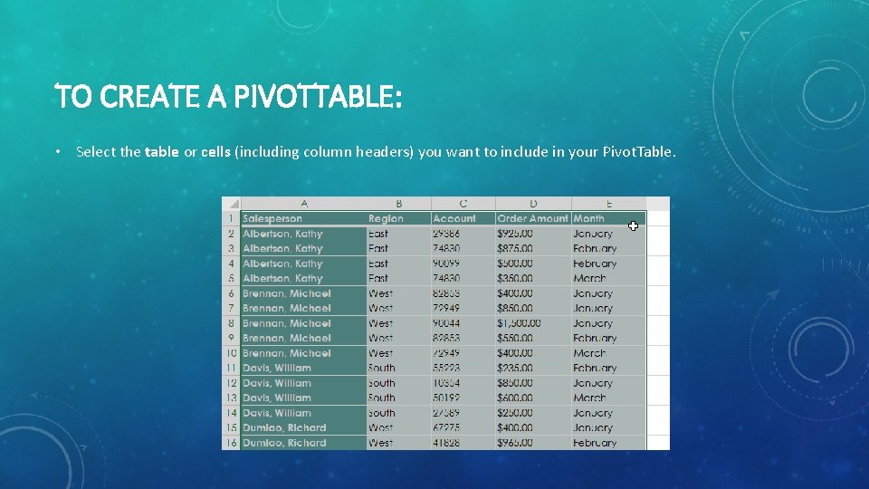
TO CREATE A PIVOTTABLE: • Select the table or cells (including column headers) you want to include in your Pivot. Table.

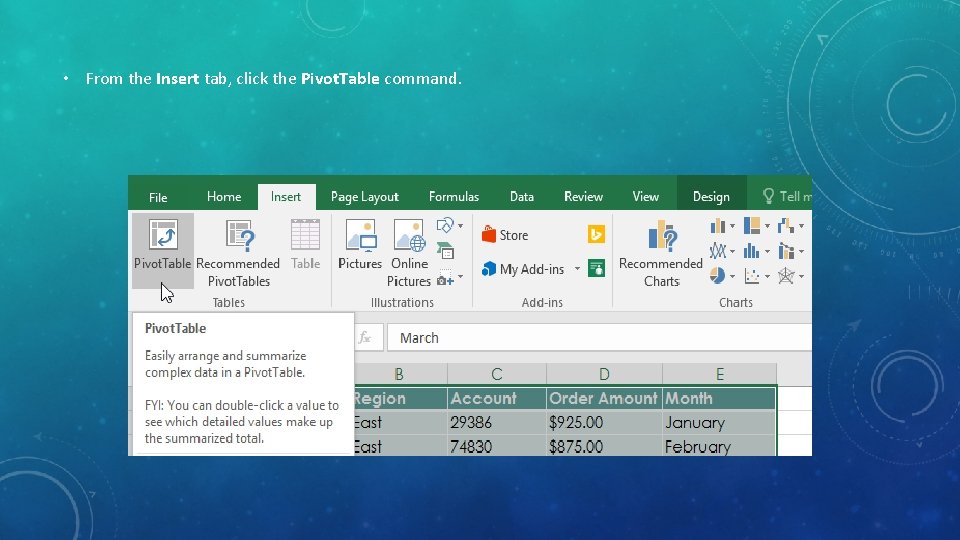
• From the Insert tab, click the Pivot. Table command.

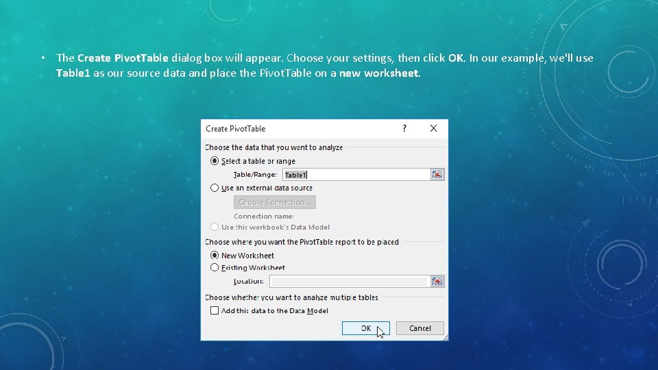
• The Create Pivot. Table dialog box will appear. Choose your settings, then click OK. In our example, we'll use Table 1 as our source data and place the Pivot. Table on a new worksheet.

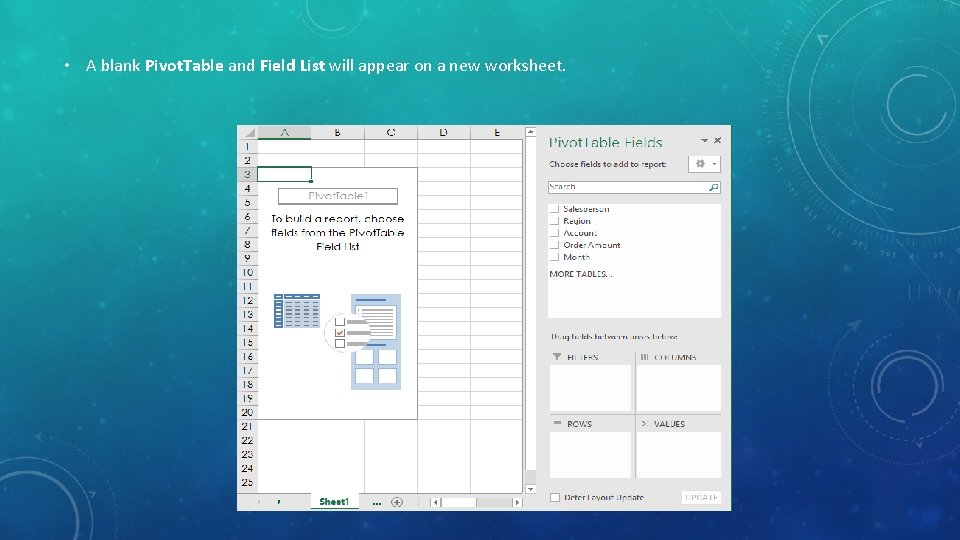
• A blank Pivot. Table and Field List will appear on a new worksheet.

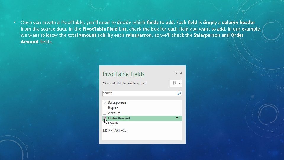
• Once you create a Pivot. Table, you'll need to decide which fields to add. Each field is simply a column header from the source data. In the Pivot. Table Field List, check the box for each field you want to add. In our example, we want to know the total amount sold by each salesperson, so we'll check the Salesperson and Order Amount fields.

• The selected fields will be added to one of the four areas below. • In our example, the Salesperson field has been added to the Rows area, while Order Amount has been added to Values. • Alternatively, you can drag and drop fields directly into the desired area.

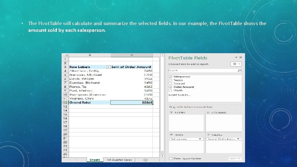
• The Pivot. Table will calculate and summarize the selected fields. In our example, the Pivot. Table shows the amount sold by each salesperson.

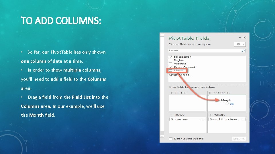
TO ADD COLUMNS: • So far, our Pivot. Table has only shown one column of data at a time. • In order to show multiple columns, you'll need to add a field to the Columns area. • Drag a field from the Field List into the Columns area. In our example, we'll use the Month field.

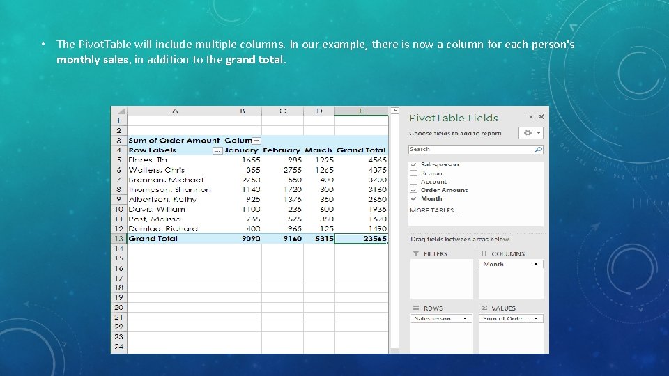
• The Pivot. Table will include multiple columns. In our example, there is now a column for each person's monthly sales, in addition to the grand total.

YOUR TASK • SHOW THE AMOUNT SOLD FOR EACH REGION.

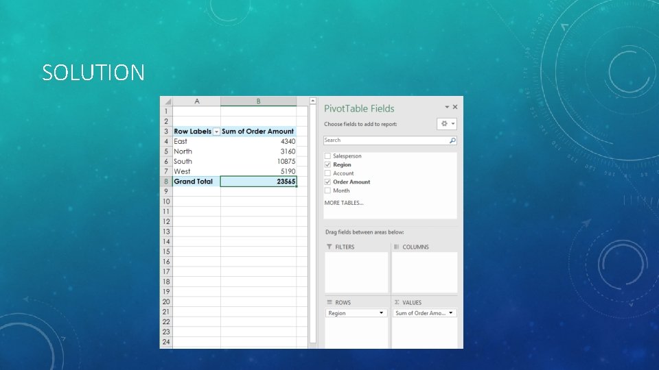
SOLUTION

YOUR TASK • In the Rows area, remove Region and replace it with Account.

YOUR TASK • Add Month to the Columns area.

YOUR TASK • Change the number format of cells B 5: E 13 to Currency. Note: You might have to make columns C and D wider in order to see the values.

SLICER IN PIVOT TABLES • Slicers make filtering data in Pivot. Tables even easier. Slicers are basically just filters but are easier and faster to use, allowing you to instantly pivot your data. If you frequently filter your Pivot. Tables, you may want to consider using slicers instead of filters.

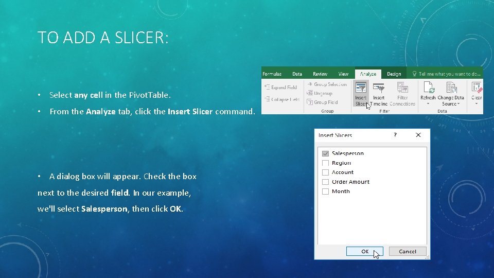
TO ADD A SLICER: • Select any cell in the Pivot. Table. • From the Analyze tab, click the Insert Slicer command. • A dialog box will appear. Check the box next to the desired field. In our example, we'll select Salesperson, then click OK.

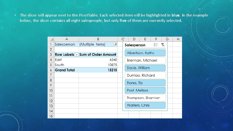
• The slicer will appear next to the Pivot. Table. Each selected item will be highlighted in blue. In the example below, the slicer contains all eight salespeople, but only five of them are currently selected.

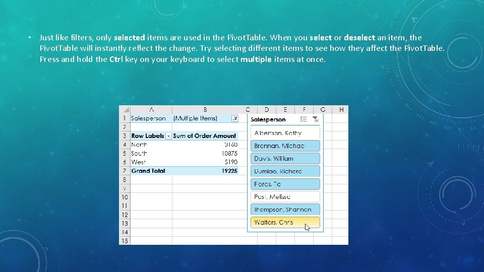
• Just like filters, only selected items are used in the Pivot. Table. When you select or deselect an item, the Pivot. Table will instantly reflect the change. Try selecting different items to see how they affect the Pivot. Table. Press and hold the Ctrl key on your keyboard to select multiple items at once.