Pipe Network Analysis A pipe network is analyzed

Pipe Network Analysis A pipe network is analyzed for the determination of the nodal pressure heads and the link discharges. The network is analyzed for the worst combination of discharge withdrawals that may result in low pressure heads in some areas. Pipe Network Geometry The water distribution networks have mainly the following three types of configurations: 1 -branched or tree-like configuration 2 - looped configuration 3 - branched and looped configuration Analysis of Looped Networks Analysis of a looped network consists of the determination of pipe discharges and the nodal heads. The following laws are used: 1 - the algebraic sum of inflow and outflow discharges at node is zero. 2 - the algebraic sum of the head loss around a loop is zero. The most commonly used looped network analysis methods are:

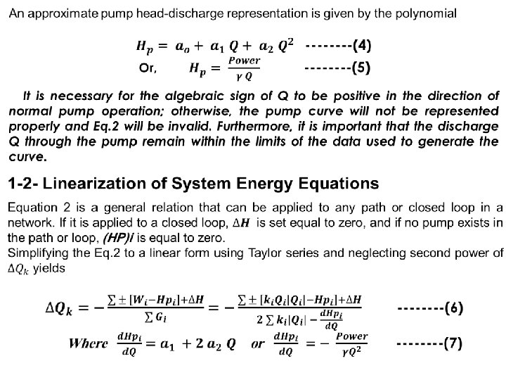
1 - Hardy Cross Method The following figure shows a relatively simple network consisting of seven pipes, two reservoirs, and one pump. The hydraulic grade lines at A and F are assumed known; these locations are termed fixed-grade nodes. Outflow demands are present at nodes C and D. Nodes C and D, along with nodes B and E are called interior nodes or junctions. Flow directions, even though not initially known, are assumed to be in the directions shown. 1 -1 - Generalized Network Equations Networks of piping, such as those shown in the figure can be represented by the following equations. 1. Continuity at the jth interior node: in which the subscript j refers to the pipes connected to a node, and Qe is the external. Use the positive sign for flow into the junction, and the negative sign for flow out of the junction. Representative piping network: (a) assumed flow directions and numbering scheme (b) designated interior loops (c) path between two fixed-grade nodes

P = J + L + F – 1 -------(3) In the figure above note that , J = 4, L = 2, F = 2, so that P = 4 + 2 -1 = 7

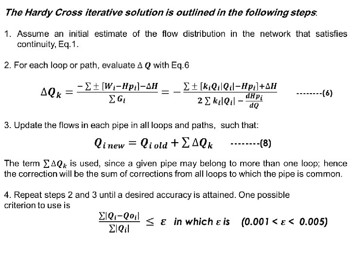
Example 1: The pipe network of two loops as shown in Fig. 3. 11 has to be analyzed by the Hardy Cross method for pipe flows for given pipe lengths L and pipe diameters D. The nodal inflow at node 1 and nodal outflow at node 3 are shown in the figure. Assume a constant friction factor f = 0. 02. Solution There are four junctions (J = 4), five pipes (P = 5), and (F= 0). Hence the number of closed loops is : L = P - J - F + 1 L = 5 - 4 - 0 + 1 = 2. The two loops and the assumed flow directions are as shown. Equation 6 is applied to each loop as follows: To apply continuity equation for initial pipe discharges, the discharges in pipes 1 and 5 equal to 0. 1 m 3/s are assumed. The obtained discharges are Q 1 = 0. 1 m 3/s (flow from node 1 to node 2) Q 2 = 0. 1 m 3/s (flow from node 2 to node 3) Q 3 = 0. 4 m 3/s (flow from node 4 to node 3) Q 4 = 0. 4 m 3/s (flow from node 1 to node 4) Q 5 = 0. 1 m 3/s (flow from node 1 to node 3)

Example 2: For the piping system shown below, determine the flow distribution and piezometric heads at the junctions using the Hardy Cross method of solution Solution There are five junctions (J = 5), eight pipes (P = 8), and two fixed-grade nodes (F= 2). Hence the number of closed loops is : L = P - J - F + 1 L = 8 - 5 - 2 + 1 = 2, plus one pseudo loop. The three loops and the assumed flow directions are as shown. Equation 6 is applied to each loop as follows:

Example 3: Re solve example 2 considering a pump located at pipe 1 with Hp = 250 – 0. 4 Q – 0. 1 Q 2 Solution

Example 4: Re solve example 2 considering a pump located at pipe 4 with Hp = 250 – 0. 4 Q – 0. 1 Q 2 Solution

Example 5: Find the water flow distribution in the parallel system shown in figure below. The pump Power is 799. 68 Kw. There are two junction (J = 1), four pipes (P = 4), and two fixed-grade nodes (F= 2). Hence the number of closed loops is : L = P - J - F + 1 L = 4 - 1 - 2 + 1 = 2. There is one pseudo loop only (F-1) only. The pseudo loop and the assumed flow directions are as shown. Equation 6 is applied to each loop as follows: [I] [III] Pipe L (m) D (mm) f ∑K 1 100 1200 0. 015 2 2 1000 0. 020 3 3 1500 0. 018 2 4 800 750 0. 021 4

Example 6: For the piping system shown below, determine the flow distribution and piezometric heads at the junction J using the Hardy Cross method of solution Solution There are one junction (J = 1), three pipes (P = 3), and three fixed-grade nodes (F= 3). Hence the number of closed loops is : L = P - J - F + 1 L = 3 - 1 - 3 + 1 = 0. There are two pseudo loop (F-1) only. The two pseudo loop and the assumed flow directions are as shown. Equation 6 is applied to each loop as follows: [1] [2] Pipe L (m) D (m) f 1 1500 0. 3 0. 01 0 2 1500 0. 3 0. 01 0 3 1500 0. 3 0. 01 0

Example 7: For the piping system shown below, determine the flow distribution and piezometric heads at the junction J using the Hardy Cross method of solution Solution There are one junction (J = 1), three pipes (P = 3), and three fixed-grade nodes (F= 3). Hence the number of closed loops is : L = P - J - F + 1 L = 3 - 1 - 3 + 1 = 0. There are two pseudo loop (F-1) only. The two pseudo loop and the assumed flow directions are as shown. Equation 6 is applied to each loop as follows: [1] [2] Pipe L (m) D (m) f 1 50 0. 15 0. 02 2 2 100 0. 10 0. 015 1 3 300 0. 10 0. 025 1

Example 8: Determine the flow distribution of water in the system shown in Fig. Assume constant friction factors, with f 0. 02. The head-discharge relation for the pump is HP = 60 -10 Q 2. Solution junctions (J = 2), pipes (P = 5), and fixed-grade nodes (F= 3). Hence the number of closed loops is : L =P -J-F+1 L = 5 - 2 - 3 + 1 = 1. There are two pseudo loop (F 1) only. The two pseudo loop and the assumed flow directions are as shown. Equation 6 is applied to each loop as follows: [2] [1] [3]