Pipe Flow Major and Minor Losses PUJA UPADHYAY

Pipe Flow: Major and Minor Losses PUJA UPADHYAY FLORIDA CENTER FOR ADVANCED AERO-PROPULSION

Pipe Flow: Major and Minor Losses Summary • When a gas or a liquid flows through a pipe, there is a loss of pressure in the fluid • Energy is required to overcome the viscous or frictional forces exerted by the walls of the pipe on the moving fluid • Flow also loses energy (or pressure) as it goes through fittings, such as valves, elbows, contractions and expansions • Minor losses are mainly due to the fact that flow separates locally as it moves through such fittings • The pressure loss in pipe flows is commonly referred to as head loss. • The frictional losses are referred to as major losses (hl) while losses through valves, fittings, etc. are called minor losses (hlm). • Together they make up the total head losses (hl. T) for pipe flows • How do we conveniently estimate pressure drop or head loss for pipes with various components and various types of flow field?

Motivation- Why? 1. Piping systems are encountered in everyday lives. For eg. Heating and cooling applications, fluid distribution networks (industrial or household). 2. Valves (control valve, needle valves, check valve, ball valves, etc), pipe fittings (elbows, tees, bends, etc. ) 3. What pressure drop is needed to drive the flow? 4. The pressure drop encountered is then used to determine the pumping requirements (space requirement, budget, flow rate requirement) 5. To estimate the amount of pressure loss that will occur for x kind of fluid with a y velocity and a, b, c properties in a pipe of length (L) and diameter (d). The piping system will have a combinations of things listed in part 2. - Alternatively, knowing the pressure drop through various element, how much pumping power is required to get the desired flow rate. Remember rating and sizing problems

Why do we need experimental results? - Limited analytical solutions available even though theory is well understood. (Pipe flow- fully developed solution for laminar flow) - Solutions are available for much simpler cases such as fully developed laminar flow in a circular pipe. - Limited opportunities for plugging in the numbers to get the “right” answer. - Dependency on experiments/ empirical relations to estimate the required parameters

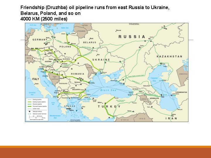
Friendship (Druzhba) oil pipeline runs from east Russia to Ukraine, Belarus, Poland, and so on 4000 KM (2500 miles)

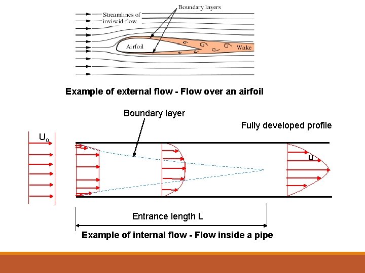
External versus Internal Flow - Flow is completely confined/bounded on all sides. Eg: Pipe Flows, blood flow inside arteries, etc. . The growth of boundary layer is confined! External Flow - Flow over bodies immersed in an unbounded fluid Eg: flow over an airfoil or turbine blades, channel flows, jets, and so on.

Example of external flow - Flow over an airfoil Boundary layer Fully developed profile Uo u Entrance length L Example of internal flow - Flow inside a pipe

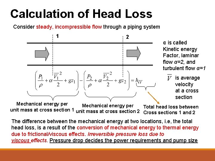
Calculation of Head Loss Consider steady, incompressible flow through a piping system 1 2 α is called Kinetic energy Factor, laminar flow α=2, and turbulent flow α=1 is average velocity at a cross section Mechanical energy per Total head loss between unit mass at cross section 1 unit mass at cross section 2 Cross sections 1 and 2 The difference between the mechanical energy at two locations, i. e, the total head loss, is a result of the conversion of mechanical energy to thermal energy due to frictional/viscous effects. Irreversible pressure loss due to viscous effects. Pressure drop decides the power requirements and pump size

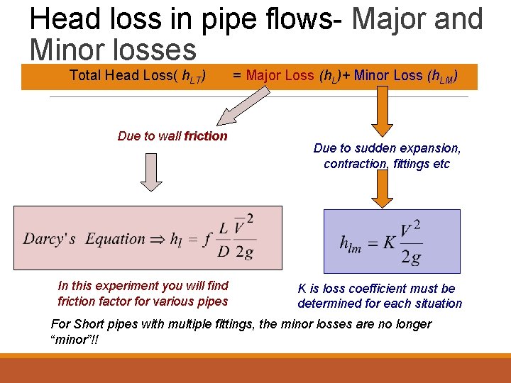
Head loss in pipe flows- Major and Minor losses Total Head Loss( h. LT) = Major Loss (h. L)+ Minor Loss (h. LM) Due to wall friction In this experiment you will find friction factor for various pipes Due to sudden expansion, contraction, fittings etc K is loss coefficient must be determined for each situation For Short pipes with multiple fittings, the minor losses are no longer “minor”!!

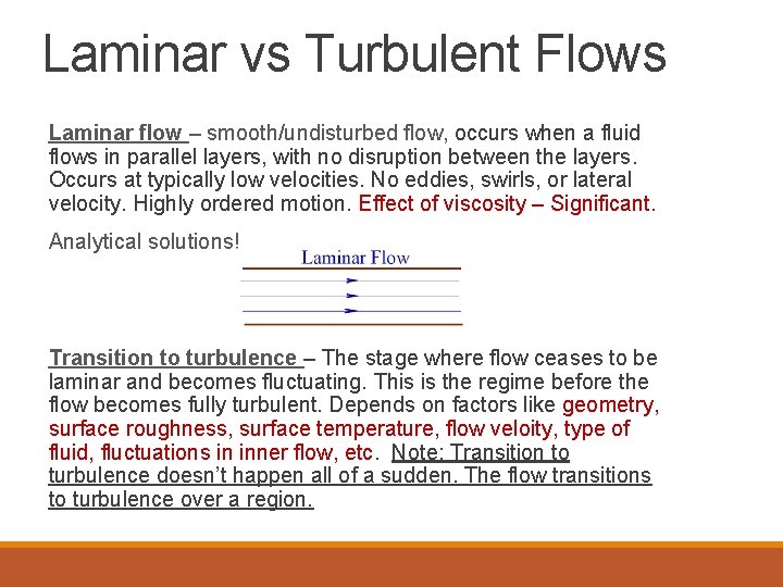
Laminar vs Turbulent Flows Laminar flow – smooth/undisturbed flow, occurs when a fluid flows in parallel layers, with no disruption between the layers. Occurs at typically low velocities. No eddies, swirls, or lateral velocity. Highly ordered motion. Effect of viscosity – Significant. Analytical solutions! Transition to turbulence – The stage where flow ceases to be laminar and becomes fluctuating. This is the regime before the flow becomes fully turbulent. Depends on factors like geometry, surface roughness, surface temperature, flow veloity, type of fluid, fluctuations in inner flow, etc. Note: Transition to turbulence doesn’t happen all of a sudden. The flow transitions to turbulence over a region.

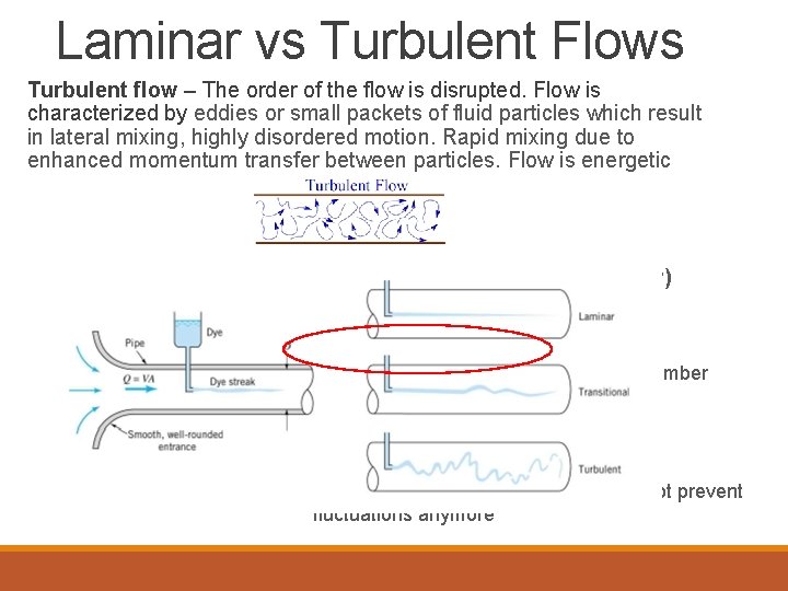
Laminar vs Turbulent Flows Turbulent flow – The order of the flow is disrupted. Flow is characterized by eddies or small packets of fluid particles which result in lateral mixing, highly disordered motion. Rapid mixing due to enhanced momentum transfer between particles. Flow is energetic Measure of flow regime – Reynolds number (Re = ρVD/µ = VD/ν) • Ratio of inertial to viscous forces Re = ρVavg. D/µ = Vavg. D/ν Effect of viscosity becomes less significant with increasing Re number μ = kg/s. m (dynamic or absolute viscosity) ν = μ/ρ = m 2/s (kinematic viscosity) High Re = low viscous forces, less orderly flow. Viscous forces cannot prevent fluctuations anymore

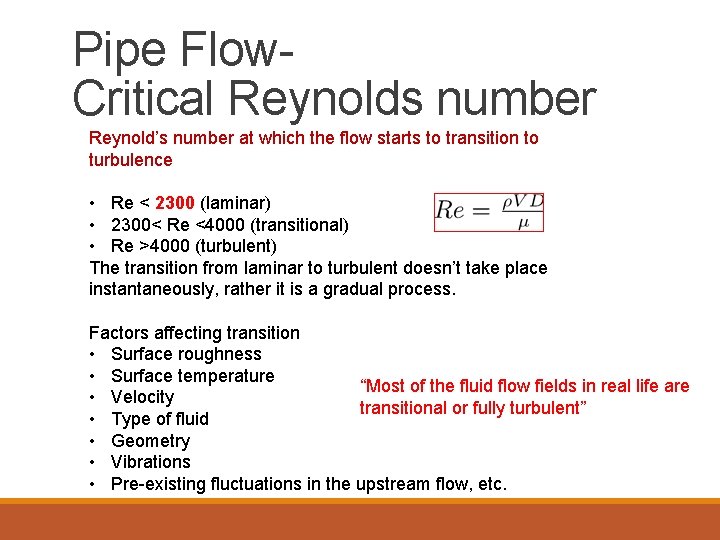
Pipe Flow- Critical Reynolds number Reynold’s number at which the flow starts to transition to turbulence • Re < 2300 (laminar) • 2300< Re <4000 (transitional) • Re >4000 (turbulent) The transition from laminar to turbulent doesn’t take place instantaneously, rather it is a gradual process. Factors affecting transition • Surface roughness • Surface temperature “Most of the fluid flow fields in real life are • Velocity transitional or fully turbulent” • Type of fluid • Geometry • Vibrations • Pre-existing fluctuations in the upstream flow, etc.

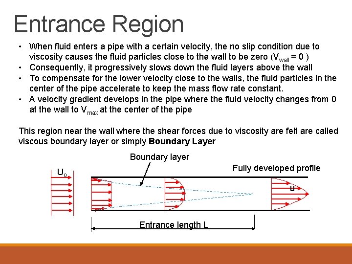
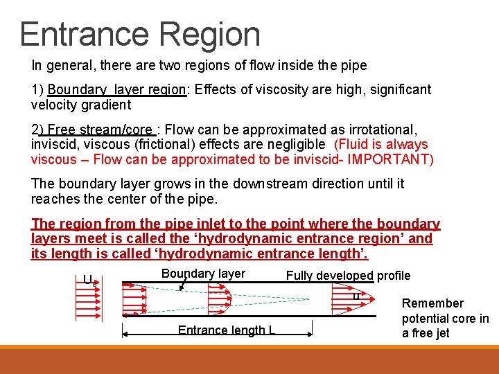
Entrance Region • When fluid enters a pipe with a certain velocity, the no slip condition due to viscosity causes the fluid particles close to the wall to be zero (Vwall = 0 ) • Consequently, it progressively slows down the fluid layers above the wall • To compensate for the lower velocity close to the walls, the fluid particles in the center of the pipe accelerate to keep the mass flow rate constant. • A velocity gradient develops in the pipe where the fluid velocity changes from 0 at the wall to Vmax at the center of the pipe This region near the wall where the shear forces due to viscosity are felt are called viscous boundary layer or simply Boundary Layer Boundary layer Fully developed profile Uo u Entrance length L

Entrance Region In general, there are two regions of flow inside the pipe 1) Boundary layer region: Effects of viscosity are high, significant velocity gradient 2) Free stream/core : Flow can be approximated as irrotational, inviscid, viscous (frictional) effects are negligible (Fluid is always viscous – Flow can be approximated to be inviscid- IMPORTANT) The boundary layer grows in the downstream direction until it reaches the center of the pipe. The region from the pipe inlet to the point where the boundary layers meet is called the ‘hydrodynamic entrance region’ and its length is called ‘hydrodynamic entrance length’. Uo Boundary layer Fully developed profile u Entrance length L Remember potential core in a free jet

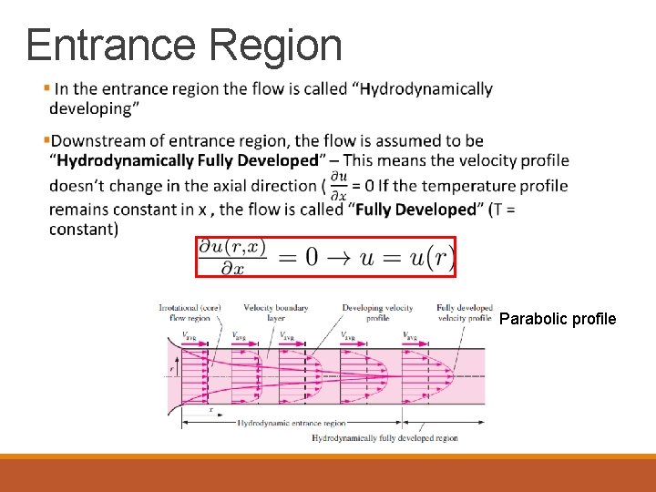
Entrance Region Parabolic profile

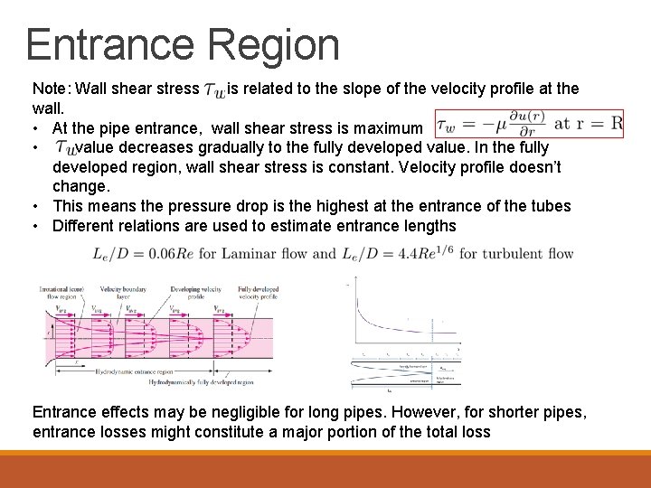
Entrance Region Note: Wall shear stress is related to the slope of the velocity profile at the wall. • At the pipe entrance, wall shear stress is maximum • value decreases gradually to the fully developed value. In the fully developed region, wall shear stress is constant. Velocity profile doesn’t change. • This means the pressure drop is the highest at the entrance of the tubes • Different relations are used to estimate entrance lengths Entrance effects may be negligible for long pipes. However, for shorter pipes, entrance losses might constitute a major portion of the total loss

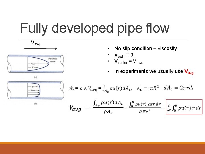
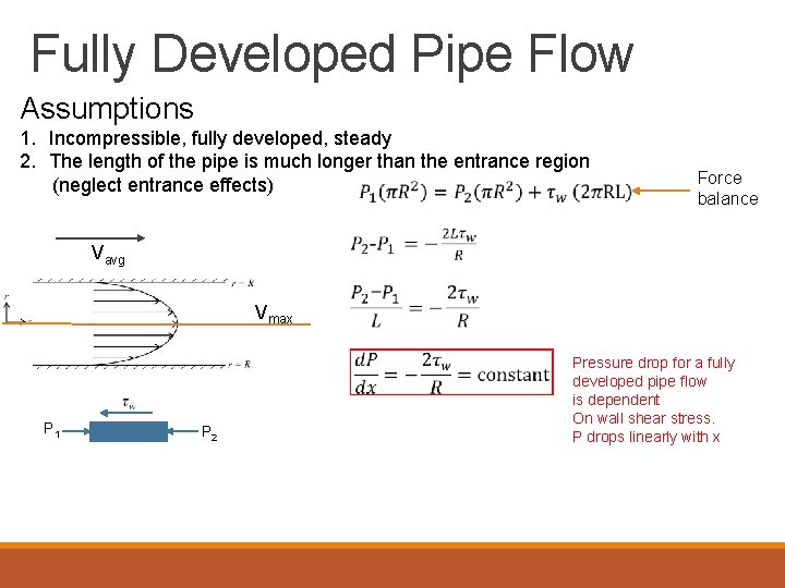
Fully developed pipe flow Vavg • No slip condition – viscosity • Vwall = 0 • Vcenter = Vmax • In experiments we usually use Vavg

Fully Developed Pipe Flow Assumptions 1. Incompressible, fully developed, steady 2. The length of the pipe is much longer than the entrance region (neglect entrance effects) Force balance Vavg Vmax P 1 P 2 Pressure drop for a fully developed pipe flow is dependent On wall shear stress. P drops linearly with x

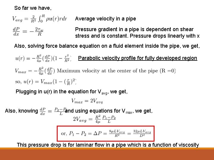
So far we have, Average velocity in a pipe Pressure gradient in a pipe is dependent on shear stress and is constant. Pressure drops linearly with x Also, solving force balance equation on a fluid element inside the pipe, we get, Parabolic velocity profile for fully developed region Plugging in u(r) in the equation for Vavg, we get, Also, knowing and using equations for Vmax, we get, This pressure drop is for laminar flow in a pipe which is a function of viscosity

What do you do for turbulent flows where analytical solutions are not available? This is when use of empirical relations become necessary. Also, a general formulation in terms of non-dimensional quantities will be helpful even for laminar flows

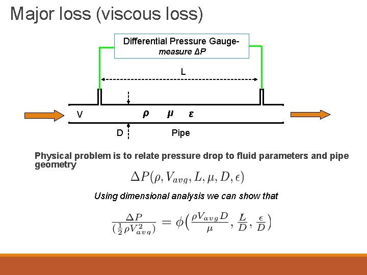
Major loss (viscous loss) Differential Pressure Gauge- measure ΔP L ρ V D μ ε Pipe Physical problem is to relate pressure drop to fluid parameters and pipe geometry Using dimensional analysis we can show that

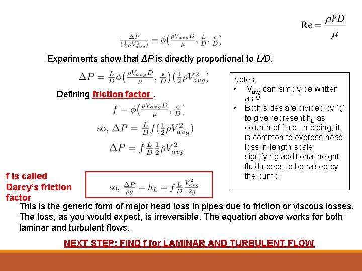
Experiments show that ΔP is directly proportional to L/D, Defining friction factor , Notes: • Vavg can simply be written as V • Both sides are divided by ’g’ to give represent h. L as column of fluid. In piping, it is common to express head loss in length scale signifying additional height fluid needs to be raised by the pump f is called Darcy’s friction factor This is the generic form of major head loss in pipes due to friction or viscous losses. The loss, as you would expect, is irreversible. The equation above works for both laminar and turbulent flows. NEXT STEP: FIND f for LAMINAR AND TURBULENT FLOW

Friction factor– Laminar Flow Generic equation for major loss From analytical solution for laminar flow, Using above equations, we can show, Where, , friction factor is only a function of Reynold’s number and NOT surface roughness, ε(Only for Laminar flow (Re < 2300). The friction factor can also be written in terms of wall shear stress for laminar pipe flow as, (Darcy’s friction factor) (Fanning friction factor)

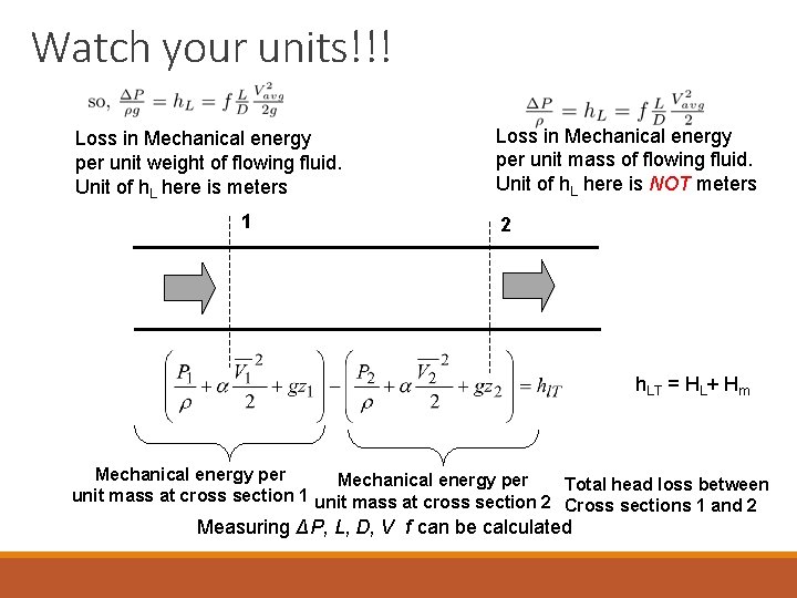
Watch your units!!! Loss in Mechanical energy per unit weight of flowing fluid. Unit of h. L here is meters 1 Loss in Mechanical energy per unit mass of flowing fluid. Unit of h. L here is NOT meters 2 h. LT = HL+ Hm Mechanical energy per Total head loss between unit mass at cross section 1 unit mass at cross section 2 Cross sections 1 and 2 Measuring ΔP, L, D, V f can be calculated

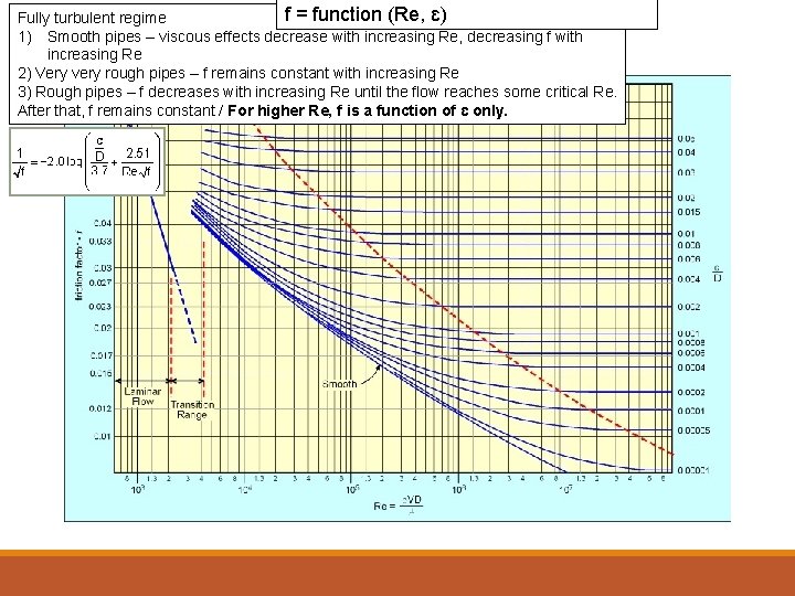
Friction Factor – Turbulent Flows • • For Turbulent flow ( Re>4000) it is not possible to derive analytical expressions. Empirical expressions relating friction factor, Reynolds number and relative roughness are available in literature In general, the friction factor f is determined experimentally and is usually published in graphical form as a function of Reynolds number and non dimensional surface Roughness ε/D. L F Moody published this data first, usually referred to as Moody’s chart

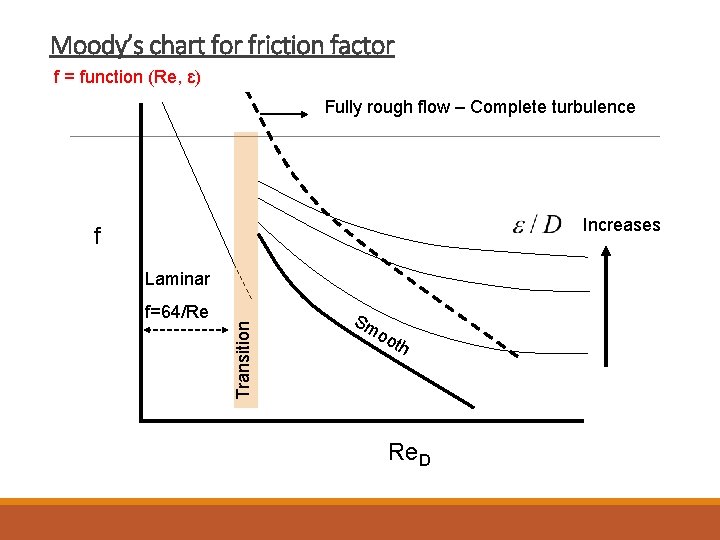
Moody’s chart for friction factor f = function (Re, ɛ) Fully rough flow – Complete turbulence Increases f f=64/Re Transition Laminar Sm oo th Re. D

f = function (Re, ɛ) Fully turbulent regime Laminar Flow: f = 64/Re (Re increases = viscous effect 1) Smooth pipes – viscous effects decrease with increasing Re, decreasing f with Transitional Regime : Critical, need experimental results decreases = smaller head loss coefficient increasing Re 2) Very very rough pipes – f remains constant with increasing Re 3) Rough pipes – f decreases with increasing Re until the flow reaches some critical Re. After that, f remains constant / For higher Re, f is a function of ɛ only.

Friction factor correlations f is not related explicitly Re and relative roughness in this equation. The following equation can be used instead

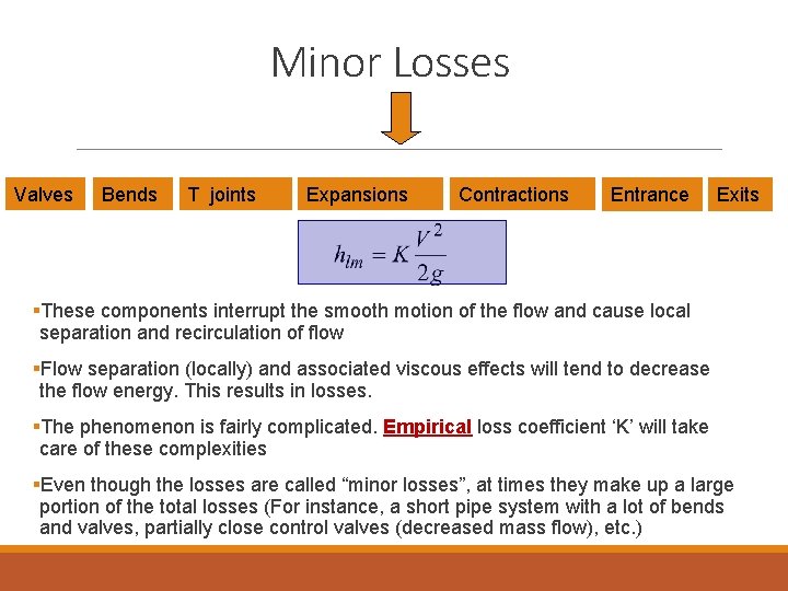
Minor Losses Valves Bends T joints Expansions Contractions Entrance Exits §These components interrupt the smooth motion of the flow and cause local separation and recirculation of flow §Flow separation (locally) and associated viscous effects will tend to decrease the flow energy. This results in losses. §The phenomenon is fairly complicated. Empirical loss coefficient ‘K’ will take care of these complexities §Even though the losses are called “minor losses”, at times they make up a large portion of the total losses (For instance, a short pipe system with a lot of bends and valves, partially close control valves (decreased mass flow), etc. )

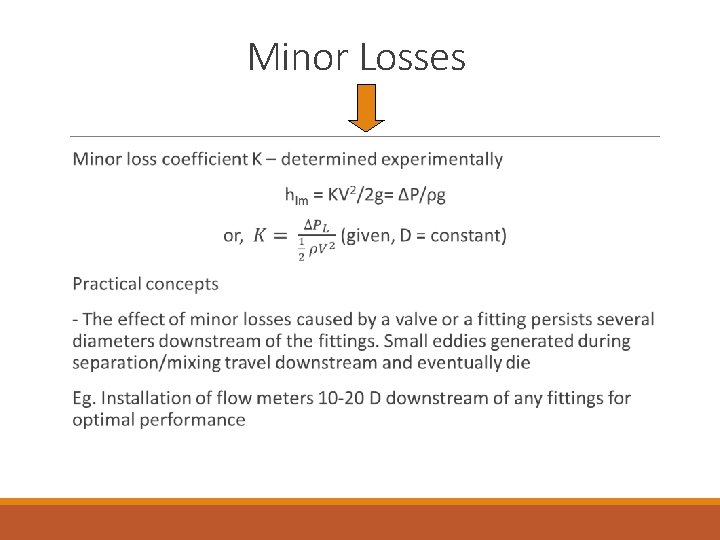
Minor Losses

Final Equation

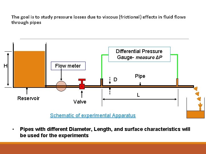
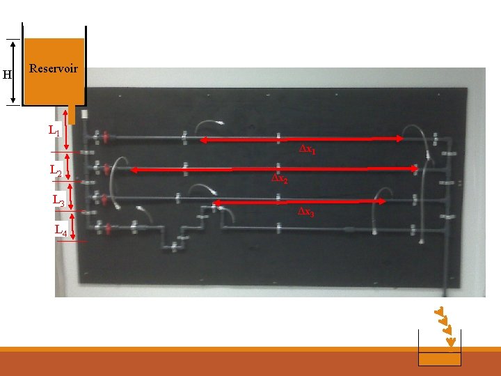
The goal is to study pressure losses due to viscous (frictional) effects in fluid flows through pipes Differential Pressure Gauge- measure ΔP Flow meter H D Reservoir Pipe L Valve Schematic of experimental Apparatus • Pipes with different Diameter, Length, and surface characteristics will be used for the experiments

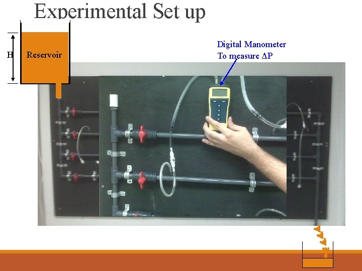
Experimental Set up H Reservoir Digital Manometer To measure ΔP

H Reservoir L 1 Δx 1 L 2 L 3 L 4 Δx 2 Δx 3