Pierre Lermusiaux Pat Haley Wayne Leslie Oleg Logoutov

Pierre Lermusiaux, Pat Haley, Wayne Leslie, Oleg Logoutov (and AWACS team) Mechanical Engineering, MIT http: //modelseas. mit. edu/ v MIT-HU AWACS Research Goals and Objectives v Selected Research Progress so far 1. Assimilation of all data sets from AWACS-SW 06 -NMFS, with real-time web-based dissemination 2. Tides/internal tides and their interactions with mesoscales: processes, modeling and predictions 3. Nested Ocean Modeling 4. Adaptive sampling with ESSE and MILP or genetic algorithms 5. Future Plans

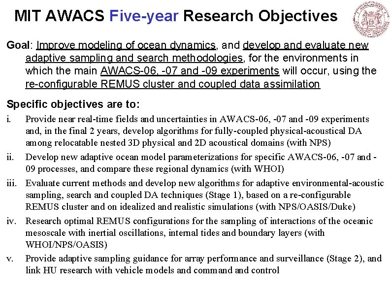
MIT AWACS Five-year Research Objectives Goal: Improve modeling of ocean dynamics, and develop and evaluate new adaptive sampling and search methodologies, for the environments in which the main AWACS-06, -07 and -09 experiments will occur, using the re-configurable REMUS cluster and coupled data assimilation Specific objectives are to: i. Provide near real-time fields and uncertainties in AWACS-06, -07 and -09 experiments and, in the final 2 years, develop algorithms for fully-coupled physical-acoustical DA among relocatable nested 3 D physical and 2 D acoustical domains (with NPS) ii. Develop new adaptive ocean model parameterizations for specific AWACS-06, -07 and 09 processes, and compare these regional dynamics (with WHOI) iii. Evaluate current methods and develop new algorithms for adaptive environmental-acoustic sampling, search and coupled DA techniques (Stage 1), based on a re-configurable REMUS cluster and on idealized and realistic simulations (with NPS/OASIS/Duke) iv. Research optimal REMUS configurations for the sampling of interactions of the oceanic mesoscale with inertial oscillations, internal tides and boundary layers (with WHOI/NPS/OASIS) v. Provide adaptive sampling guidance for array performance and surveillance (Stage 2), and link HU research with vehicle models and command control

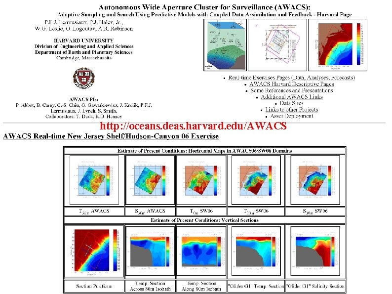
http: //oceans. deas. harvard. edu/AWACS

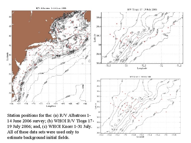
Station positions for the: (a) R/V Albatross 114 June 2006 survey; (b) WHOI R/V Tioga 1719 July 2006; and, (c) WHOI Knorr 1 -31 July. All of these data sets were used only to estimate background initial fields.

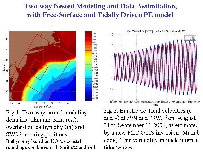
Two-way Nested Modeling and Data Assimilation, with Free-Surface and Tidally Driven PE model Fig 1. Two-way nested modeling domains (1 km and 3 km res. ), overlaid on bathymetry (m) and SW 06 mooring positions. Bathymetry based on NOAA coastal soundings combined with Smith&Sandwell Fig 2. Barotropic Tidal velocities (u and v) at 39 N and 73 W, from August 31 to September 11 2006, as estimated by a new MIT-OTIS inversion (Matlab code). This variability impacts internal tides/waves.

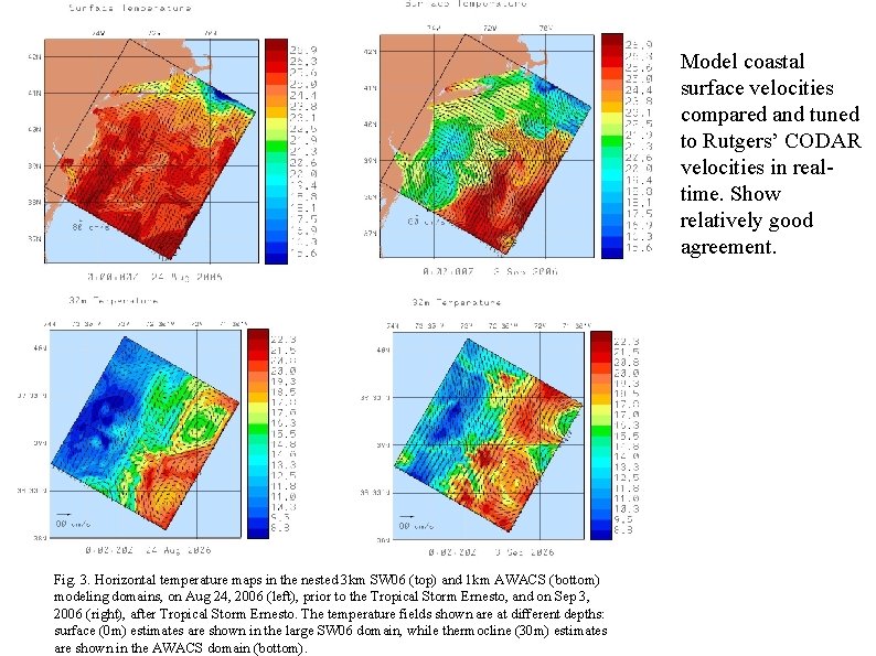
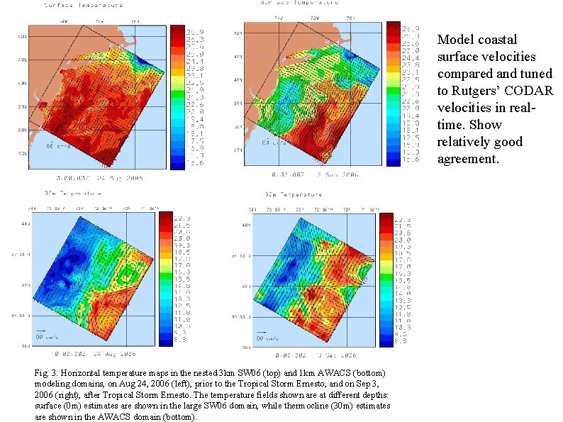
Model coastal surface velocities compared and tuned to Rutgers’ CODAR velocities in realtime. Show relatively good agreement. Fig. 3. Horizontal temperature maps in the nested 3 km SW 06 (top) and 1 km AWACS (bottom) modeling domains, on Aug 24, 2006 (left), prior to the Tropical Storm Ernesto, and on Sep 3, 2006 (right), after Tropical Storm Ernesto. The temperature fields shown are at different depths: surface (0 m) estimates are shown in the large SW 06 domain, while thermocline (30 m) estimates are shown in the AWACS domain (bottom).

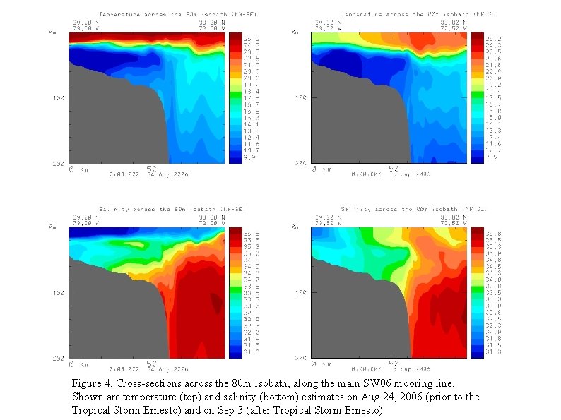
Figure 4. Cross-sections across the 80 m isobath, along the main SW 06 mooring line. Shown are temperature (top) and salinity (bottom) estimates on Aug 24, 2006 (prior to the Tropical Storm Ernesto) and on Sep 3 (after Tropical Storm Ernesto).

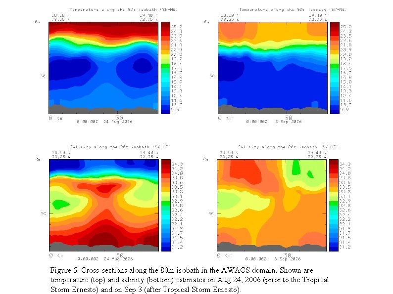
Figure 5. Cross-sections along the 80 m isobath in the AWACS domain. Shown are temperature (top) and salinity (bottom) estimates on Aug 24, 2006 (prior to the Tropical Storm Ernesto) and on Sep 3 (after Tropical Storm Ernesto).

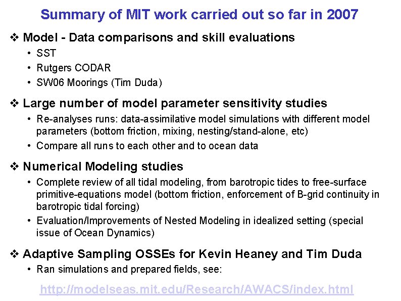
Summary of MIT work carried out so far in 2007 v Model - Data comparisons and skill evaluations • SST • Rutgers CODAR • SW 06 Moorings (Tim Duda) v Large number of model parameter sensitivity studies • Re-analyses runs: data-assimilative model simulations with different model parameters (bottom friction, mixing, nesting/stand-alone, etc) • Compare all runs to each other and to ocean data v Numerical Modeling studies • Complete review of all tidal modeling, from barotropic tides to free-surface primitive-equations model (bottom friction, enforcement of B-grid continuity in barotropic tidal forcing) • Evaluation/Improvements of Nested Modeling in idealized setting (special issue of Ocean Dynamics) v Adaptive Sampling OSSEs for Kevin Heaney and Tim Duda • Ran simulations and prepared fields, see: http: //modelseas. mit. edu/Research/AWACS/index. html

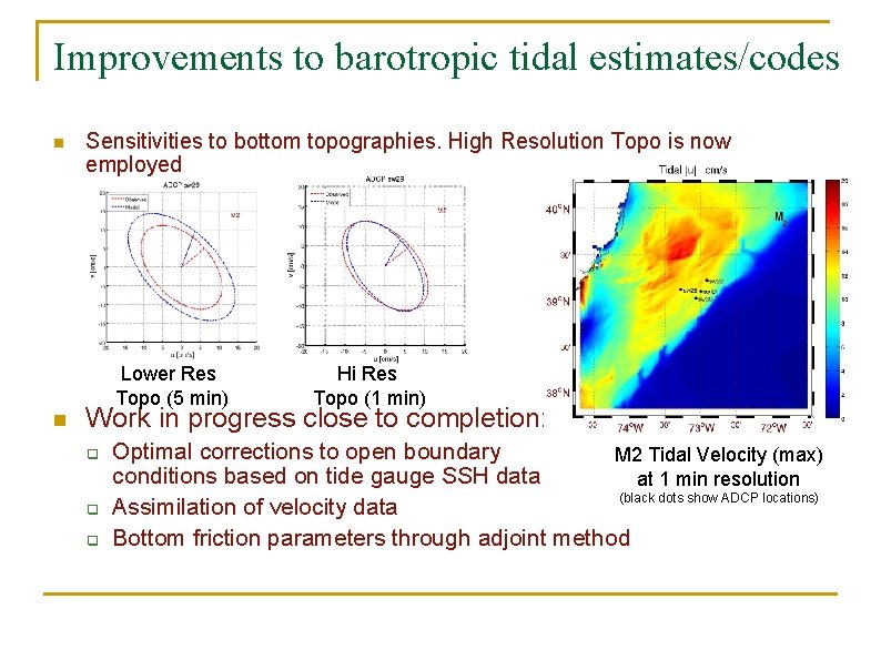
Improvements to barotropic tidal estimates/codes n Sensitivities to bottom topographies. High Resolution Topo is now employed Lower Res Topo (5 min) n Hi Res Topo (1 min) Work in progress close to completion: q q q Optimal corrections to open boundary M 2 Tidal Velocity (max) conditions based on tide gauge SSH data at 1 min resolution (black dots show ADCP locations) Assimilation of velocity data Bottom friction parameters through adjoint method

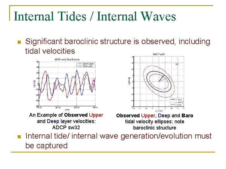
Internal Tides / Internal Waves n Significant baroclinic structure is observed, including tidal velocities An Example of Observed Upper and Deep layer velocities: ADCP sw 32 n Observed Upper, Deep and Baro tidal velocity ellipses: note baroclinic structure Internal tide/ internal wave generation/evolution must be captured

Towards Modeling and Scientific studies of Tides/internal tides and their interactions with mesoscales v Most of the MIT-AWACS 2007 work so far (with model-data comparisons) v Approach: Model estimates sampled at ½ hr intervals at selected mooring locations and compared to mooring data by Tim Duda (WHOI) v Even though results are encouraging, fine scale needs improvement ○ 1 km resolution insufficient (internal tides) ○ We are researching new adaptive sub-mesoscale parameterizations T data T Model

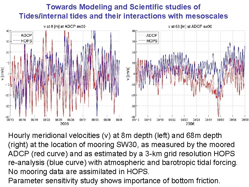
Towards Modeling and Scientific studies of Tides/internal tides and their interactions with mesoscales Hourly meridional velocities (v) at 8 m depth (left) and 68 m depth (right) at the location of mooring SW 30, as measured by the moored ADCP (red curve) and as estimated by a 3 -km grid resolution HOPS re-analysis (blue curve) with atmospheric and barotropic tidal forcing. No mooring data are assimilated in HOPS. Parameter sensitivity study shows importance of bottom friction.

Model coastal surface velocities compared and tuned to Rutgers’ CODAR velocities in realtime. Show relatively good agreement. Fig. 3. Horizontal temperature maps in the nested 3 km SW 06 (top) and 1 km AWACS (bottom) modeling domains, on Aug 24, 2006 (left), prior to the Tropical Storm Ernesto, and on Sep 3, 2006 (right), after Tropical Storm Ernesto. The temperature fields shown are at different depths: surface (0 m) estimates are shown in the large SW 06 domain, while thermocline (30 m) estimates are shown in the AWACS domain (bottom).

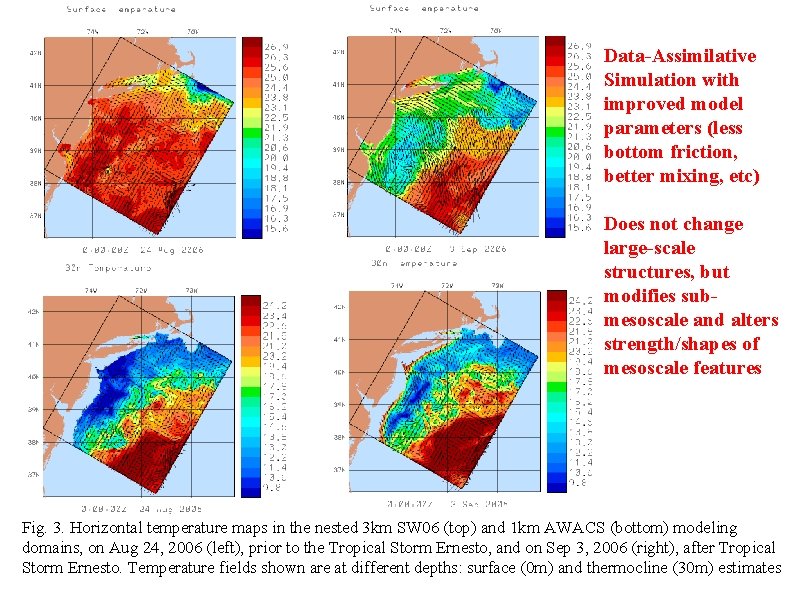
Data-Assimilative Simulation with improved model parameters (less bottom friction, better mixing, etc) Does not change large-scale structures, but modifies submesoscale and alters strength/shapes of mesoscale features Fig. 3. Horizontal temperature maps in the nested 3 km SW 06 (top) and 1 km AWACS (bottom) modeling domains, on Aug 24, 2006 (left), prior to the Tropical Storm Ernesto, and on Sep 3, 2006 (right), after Tropical Storm Ernesto. Temperature fields shown are at different depths: surface (0 m) and thermocline (30 m) estimates

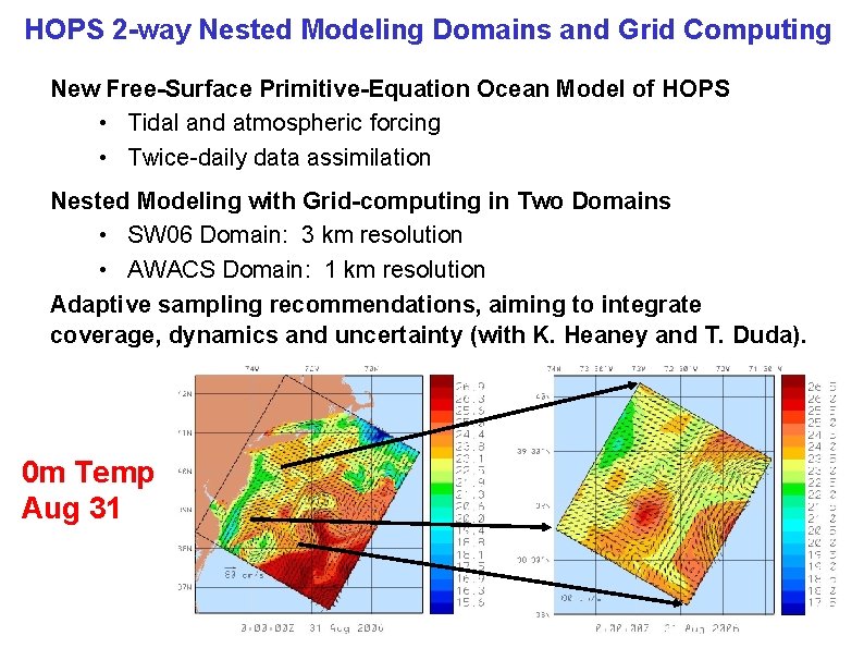
HOPS 2 -way Nested Modeling Domains and Grid Computing New Free-Surface Primitive-Equation Ocean Model of HOPS • Tidal and atmospheric forcing • Twice-daily data assimilation Nested Modeling with Grid-computing in Two Domains • SW 06 Domain: 3 km resolution • AWACS Domain: 1 km resolution Adaptive sampling recommendations, aiming to integrate coverage, dynamics and uncertainty (with K. Heaney and T. Duda). 0 m Temp Aug 31

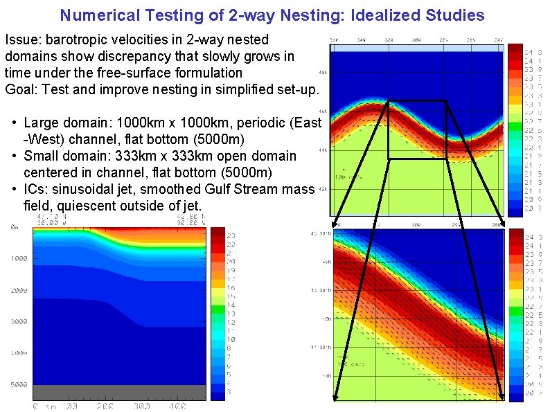
Numerical Testing of 2 -way Nesting: Idealized Studies Issue: barotropic velocities in 2 -way nested domains show discrepancy that slowly grows in time under the free-surface formulation Goal: Test and improve nesting in simplified set-up. • Large domain: 1000 km x 1000 km, periodic (East -West) channel, flat bottom (5000 m) • Small domain: 333 km x 333 km open domain centered in channel, flat bottom (5000 m) • ICs: sinusoidal jet, smoothed Gulf Stream mass field, quiescent outside of jet.

Model Output Files from Control Forecast Runs (for OSSE) In collaborations with Kevin Heaney and Tim Duda http: //modelseas. mit. edu/Research/AWACS/Run. Comp. Osse/Control/ Here we provide the output net. CDF files from a series of forecast runs for two different time periods: Prior to tropical storm Ernesto (24 -27 Aug 2007) Central Simulation After tropical storm Ernesto (4 -7 Sep 2007) Central Simulation Outputs are hourly. Each file contains temperature (°C), salinity (PSU) and horizontal velocity (cm/s, aligned East-West and North-South) fields, every hour, on the following constant depth levels (in m): 0 -5 -10 -15 -20 -25 -30 -40 -50 -60 -80 -100 -125 -150 -200 -250 -300 -400 -500 -600 -800 -1000 -1250 -1500 -2000 -2500 -3000

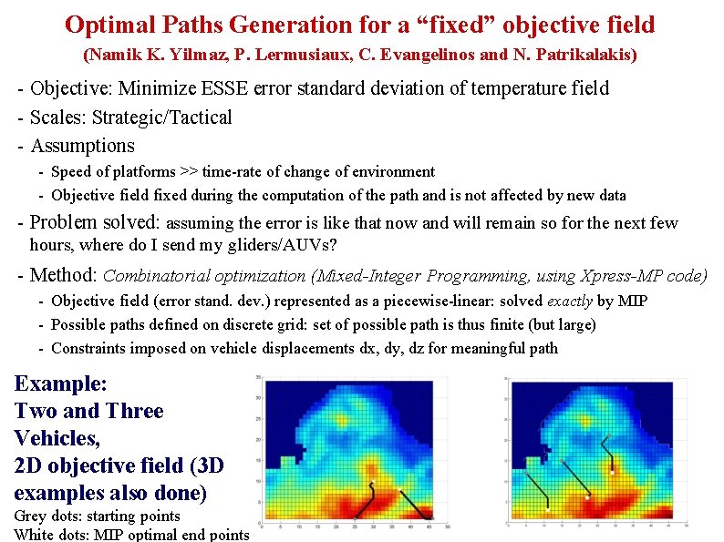
Optimal Paths Generation for a “fixed” objective field (Namik K. Yilmaz, P. Lermusiaux, C. Evangelinos and N. Patrikalakis) - Objective: Minimize ESSE error standard deviation of temperature field - Scales: Strategic/Tactical - Assumptions - Speed of platforms >> time-rate of change of environment - Objective field fixed during the computation of the path and is not affected by new data - Problem solved: assuming the error is like that now and will remain so for the next few hours, where do I send my gliders/AUVs? - Method: Combinatorial optimization (Mixed-Integer Programming, using Xpress-MP code) - Objective field (error stand. dev. ) represented as a piecewise-linear: solved exactly by MIP - Possible paths defined on discrete grid: set of possible path is thus finite (but large) - Constraints imposed on vehicle displacements dx, dy, dz for meaningful path Example: Two and Three Vehicles, 2 D objective field (3 D examples also done) Grey dots: starting points White dots: MIP optimal end points