Physics Chapter 1 Introduction Theories and Experiments n

Physics Chapter 1 Introduction

Theories and Experiments n n n The goal of physics is to develop theories based on experiments A theory is a “guess, ” expressed mathematically, about how a system works The theory makes predictions about how a system should work Experiments check theories’ predictions Every theory is a work in progress

Fundamental Quantities and Their Dimension n Length [L] meters Mass [M] kilograms Time [T] seconds n n other physical quantities can be constructed from these three These are called derived units with examples of velocity, m/s, force; kgm/s 2

Units n To communicate the result of a measurement for a quantity, a unit must be defined n n What is a gram? How long is a meter? Defining units allows everyone to relate to the same fundamental amount n How is a second defined?

Systems of Measurement n Standardized systems n n agreed upon by some authority, usually a governmental body SI -- Systéme International n n n agreed to in 1960 by an international committee main system used in this text also called mks (meter, kilogram, second) for the first letters in the units of the fundamental quantities

Systems of Measurements, cont n cgs – Gaussian system n named for the first letters of the units it uses for fundamental quantities Centimeter, gram, second US Customary n n everyday units often uses weight, in pounds, instead of mass as a fundamental quantity

Length n Units n n SI – meter, m cgs – centimeter, cm US Customary – foot, ft Defined in terms of a meter – the distance traveled by light in a vacuum during a given time of 1/299792458 second. This establishes the speed of light at 299792458 m/sec or its accepted value of 3. 00 x 108 m/s.

Mass n Units n n n SI – kilogram, kg cgs – gram, g USC – slug, slug

Standard Kilogram Defined in terms of kilogram, based on a specific cylinder of platinum and iridium alloy kept at the International Bureau of Weights and Measures located in Sevres, France.

Time n Units n n n seconds, s in all three systems 9192631700 times the period of oscillation of radiation from a cesium atom The current standard cesium clock was built and is housed at the National Institute of Standards and Technology Laboratory in Boulder, Colorado

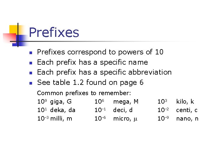
Prefixes n n Prefixes correspond to powers of 10 Each prefix has a specific name Each prefix has a specific abbreviation See table 1. 2 found on page 6 Common prefixes 109 giga, G 101 deka, da 10 -3 milli, m to remember: 106 mega, M 10 -1 deci, d 10 -6 micro, 103 10 -2 10 -9 kilo, k centi, c nano, n

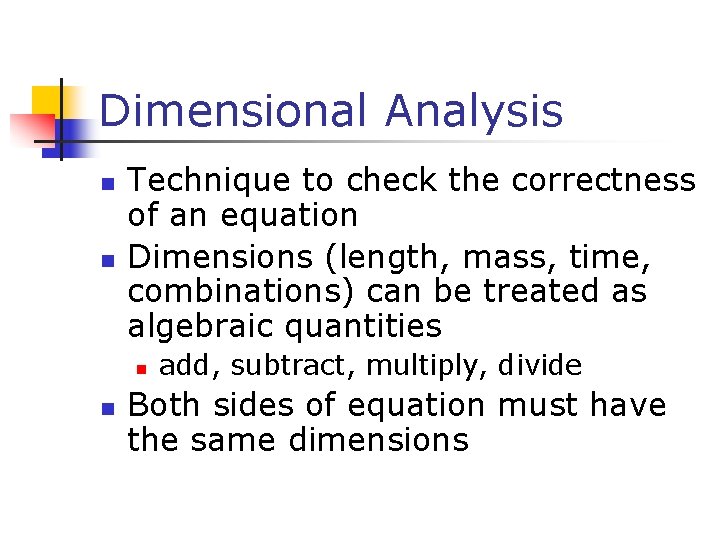
Dimensional Analysis n n Technique to check the correctness of an equation Dimensions (length, mass, time, combinations) can be treated as algebraic quantities n n add, subtract, multiply, divide Both sides of equation must have the same dimensions

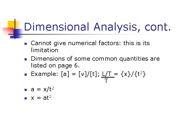
Dimensional Analysis, cont. n n n Cannot give numerical factors: this is its limitation Dimensions of some common quantities are listed on page 6. Example: [a] = [v]/[t]; L/T = {x}/{t 2} T a = x/t 2 x = at 2

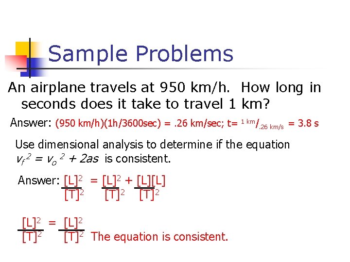
Sample Problems An airplane travels at 950 km/h. How long in seconds does it take to travel 1 km? Answer: (950 km/h)(1 h/3600 sec) =. 26 km/sec; t= 1 km/. 26 km/s = 3. 8 s Use dimensional analysis to determine if the equation vf 2 = vo 2 + 2 as is consistent. Answer: [L]2 = [L]2 + [L][L] [T]2 [L]2 = [L]2 [T]2 The equation is consistent.

Uncertainty in Measurements n There is uncertainty in every measurement, this uncertainty carries over through the calculations n n need a technique to account for this uncertainty We will use rules for significant figures to approximate the uncertainty in results of calculations

Significant Figures n n n A significant figure is one that is reliably known All non-zero digits are significant Zeros are significant when n between other non-zero digits after the decimal point and another significant figure can be clarified by using scientific notation

Operations with Significant Figures When multiplying or dividing two or more quantities, the number of significant figures in the final result is the same as the number of significant figures in the least accurate of the factors being combined

Operations with Significant Figures, cont. n n n When adding or subtracting, round the result to the smallest number of decimal places of any term in the sum If the last digit to be dropped is less than 5, drop the digit If the last digit dropped is greater than or equal to 5, raise the last retained digit by 1

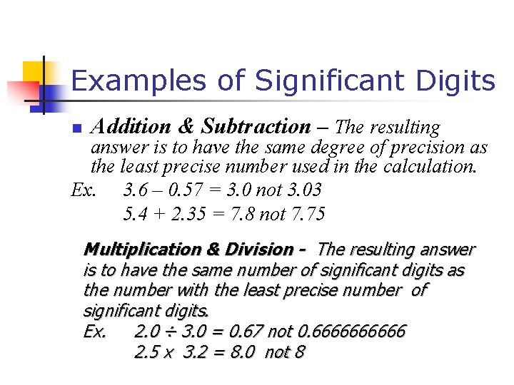
Examples of Significant Digits n Addition & Subtraction – The resulting answer is to have the same degree of precision as the least precise number used in the calculation. Ex. 3. 6 – 0. 57 = 3. 0 not 3. 03 5. 4 + 2. 35 = 7. 8 not 7. 75 Multiplication & Division - The resulting answer is to have the same number of significant digits as the number with the least precise number of significant digits. Ex. 2. 0 ÷ 3. 0 = 0. 67 not 0. 66666 2. 5 x 3. 2 = 8. 0 not 8

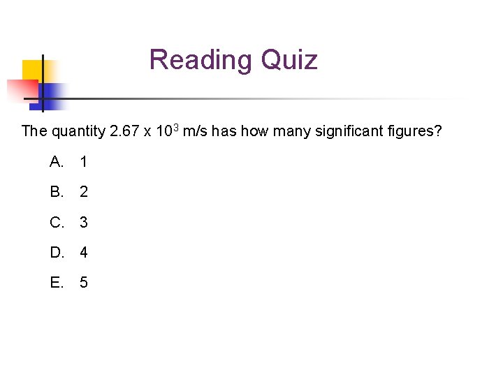
Reading Quiz The quantity 2. 67 x 103 m/s has how many significant figures? A. 1 B. 2 C. 3 D. 4 E. 5

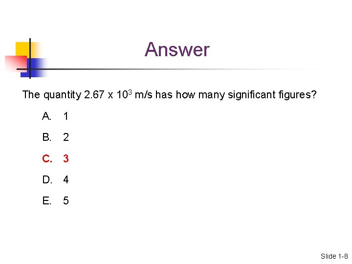
Answer The quantity 2. 67 x 103 m/s has how many significant figures? A. 1 B. 2 C. 3 D. 4 E. 5 Slide 1 -8

Importance of Measurements n n Data collection and interpretation are essential skills in physics Repeatability to obtain measurements and the degree of uncertainty of correctness are very important

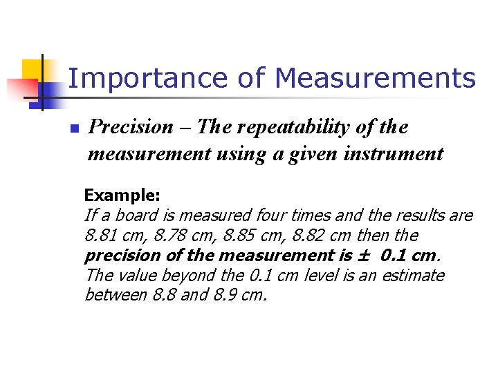
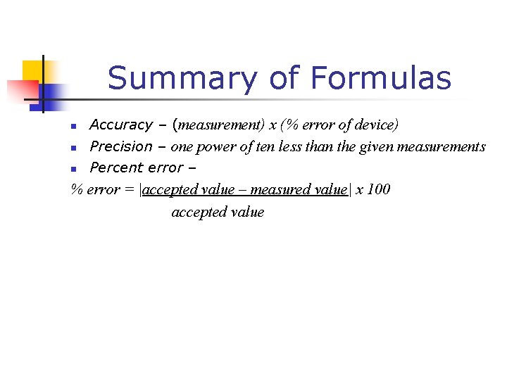
Importance of Measurements n Precision – The repeatability of the measurement using a given instrument Example: If a board is measured four times and the results are 8. 81 cm, 8. 78 cm, 8. 85 cm, 8. 82 cm then the precision of the measurement is ± 0. 1 cm. The value beyond the 0. 1 cm level is an estimate between 8. 8 and 8. 9 cm.

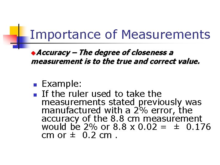
Importance of Measurements u. Accuracy – The degree of closeness a measurement is to the true and correct value. n n Example: If the ruler used to take the measurements stated previously was manufactured with a 2% error, the accuracy of the 8. 8 cm measurement would be 2% or 8. 8 x 0. 02 = ± 0. 176 cm or ± 0. 2 cm.

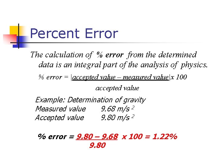
Percent Error The calculation of % error from the determined data is an integral part of the analysis of physics. % error = |accepted value – measured value|x 100 accepted value Example: Determination of gravity Measured value 9. 68 m/s 2 Accepted value 9. 80 m/s 2 % error = 9. 80 – 9. 68 x 100 = 1. 22% 9. 80

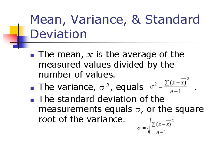
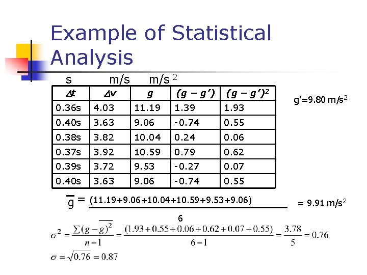
Mean, Variance, & Standard Deviation n The mean, is the average of the measured values divided by the number of values. The variance, 2, equals. The standard deviation of the measurements equals , or the square root of the variance.

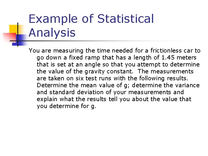
Example of Statistical Analysis You are measuring the time needed for a frictionless car to go down a fixed ramp that has a length of 1. 45 meters that is set at an angle so that you attempt to determine the value of the gravity constant. The measurements are taken on six test runs with the following results. Determine the mean value of g; determine the variance and standard deviation of your measurements and explain what the results tell you about the value that you determine for g.

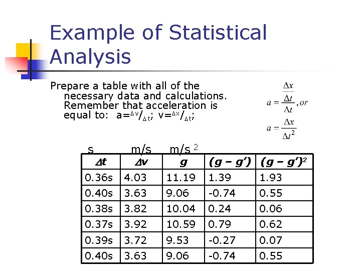
Example of Statistical Analysis Prepare a table with all of the necessary data and calculations. Remember that acceleration is equal to: a= v/ t; v= x/ t; s m/s 2 t v g (g – g’)2 0. 36 s 4. 03 11. 19 1. 39 1. 93 0. 40 s 3. 63 9. 06 -0. 74 0. 55 0. 38 s 3. 82 10. 04 0. 24 0. 06 0. 37 s 3. 92 10. 59 0. 79 0. 62 0. 39 s 3. 72 9. 53 -0. 27 0. 07 0. 40 s 3. 63 9. 06 -0. 74 0. 55

Example of Statistical Analysis s m/s 2 t v g (g – g’)2 0. 36 s 4. 03 11. 19 1. 39 1. 93 0. 40 s 3. 63 9. 06 -0. 74 0. 55 0. 38 s 3. 82 10. 04 0. 24 0. 06 0. 37 s 3. 92 10. 59 0. 79 0. 62 0. 39 s 3. 72 9. 53 -0. 27 0. 07 0. 40 s 3. 63 9. 06 -0. 74 0. 55 g = (11. 19+9. 06+10. 04+10. 59+9. 53+9. 06) 6 g’=9. 80 m/s 2 = 9. 91 m/s 2

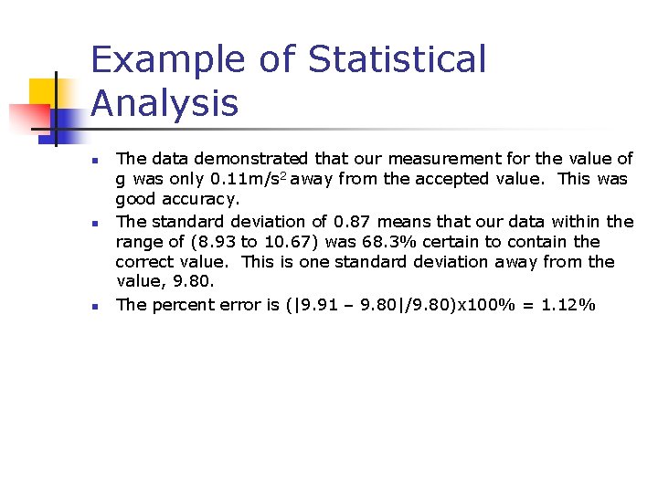
Example of Statistical Analysis n n n The data demonstrated that our measurement for the value of g was only 0. 11 m/s 2 away from the accepted value. This was good accuracy. The standard deviation of 0. 87 means that our data within the range of (8. 93 to 10. 67) was 68. 3% certain to contain the correct value. This is one standard deviation away from the value, 9. 80. The percent error is (|9. 91 – 9. 80|/9. 80)x 100% = 1. 12%

Summary of Formulas n n n Accuracy – (measurement) x (% error of device) Precision – one power of ten less than the given measurements Percent error – % error = |accepted value – measured value| x 100 accepted value

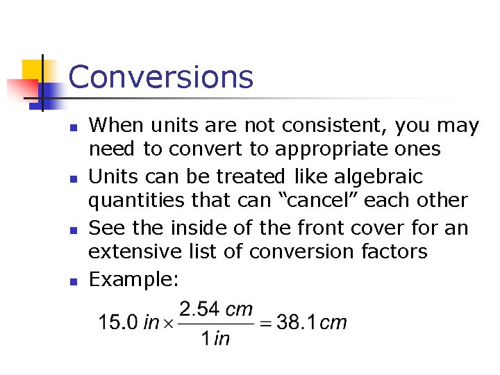
Conversions n n When units are not consistent, you may need to convert to appropriate ones Units can be treated like algebraic quantities that can “cancel” each other See the inside of the front cover for an extensive list of conversion factors Example:

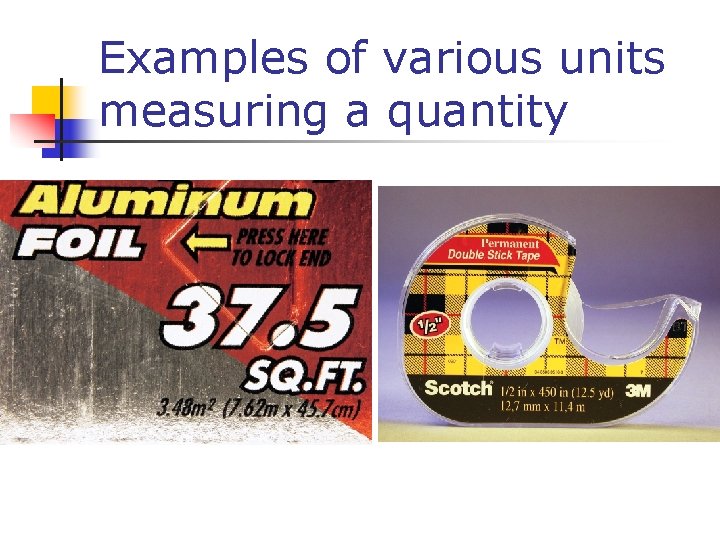
Examples of various units measuring a quantity

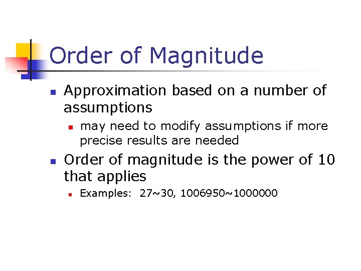
Order of Magnitude n Approximation based on a number of assumptions n n may need to modify assumptions if more precise results are needed Order of magnitude is the power of 10 that applies n Examples: 27~30, 1006950~1000000

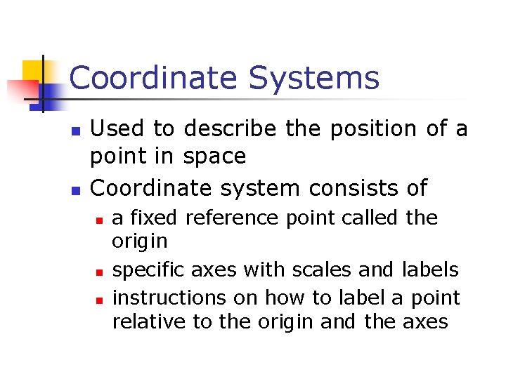
Coordinate Systems n n Used to describe the position of a point in space Coordinate system consists of n n n a fixed reference point called the origin specific axes with scales and labels instructions on how to label a point relative to the origin and the axes

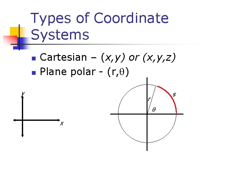
Types of Coordinate Systems n n Cartesian – (x, y) or (x, y, z) Plane polar - (r, ) y s r x

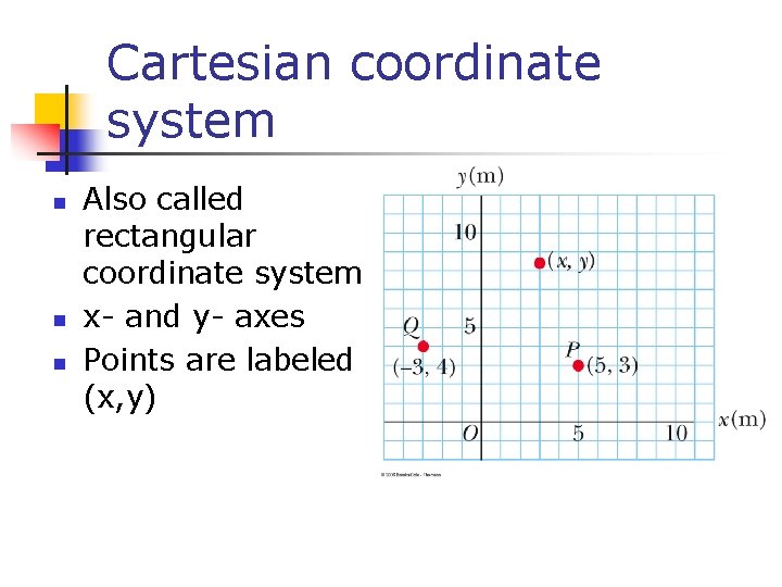
Cartesian coordinate system n n n Also called rectangular coordinate system x- and y- axes Points are labeled (x, y)

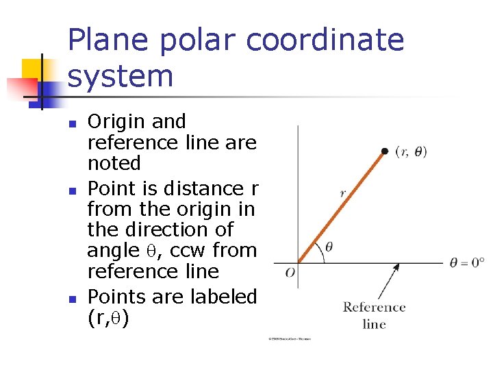
Plane polar coordinate system n n n Origin and reference line are noted Point is distance r from the origin in the direction of angle , ccw from reference line Points are labeled (r, )

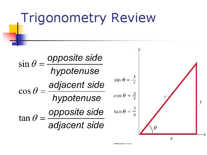
Trigonometry Review

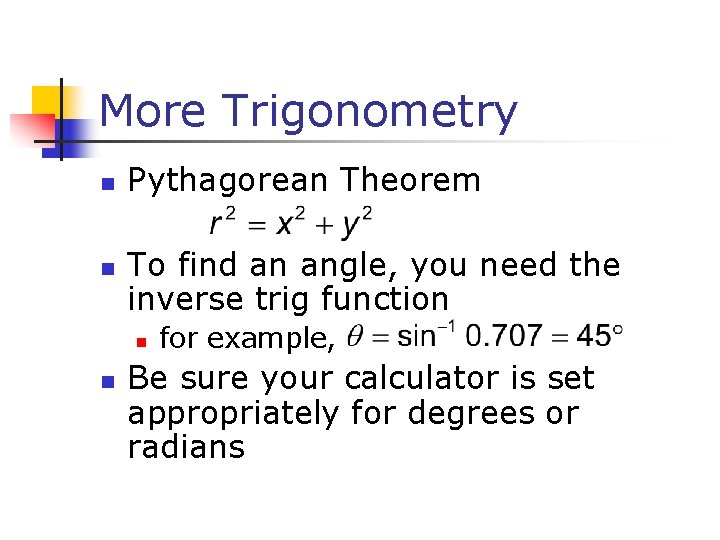
More Trigonometry n n Pythagorean Theorem To find an angle, you need the inverse trig function n n for example, Be sure your calculator is set appropriately for degrees or radians

Graphing Data n n A variable is any factor that might affect the behavior of an experimental setup. It is the key ingredient when it comes to plotting data on a graph. The independent variable is the factor that is changed or manipulated during the experiment. The dependent variable is the factor that depends on the independent variable.

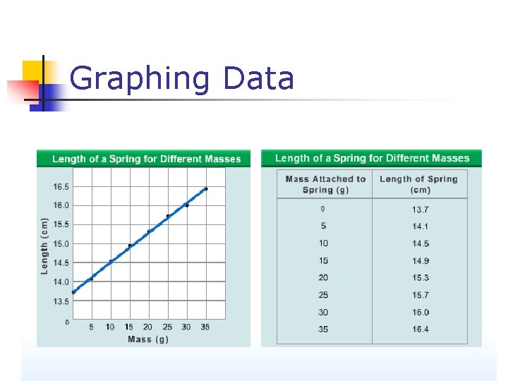
Graphing Data

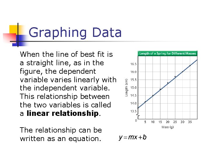
Graphing Data When the line of best fit is a straight line, as in the figure, the dependent variable varies linearly with the independent variable. This relationship between the two variables is called a linear relationship. The relationship can be written as an equation.

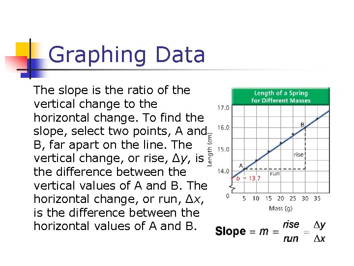
Graphing Data The slope is the ratio of the vertical change to the horizontal change. To find the slope, select two points, A and B, far apart on the line. The vertical change, or rise, Δy, is the difference between the vertical values of A and B. The horizontal change, or run, Δx, is the difference between the horizontal values of A and B.

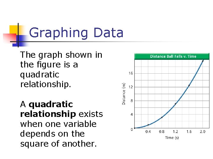
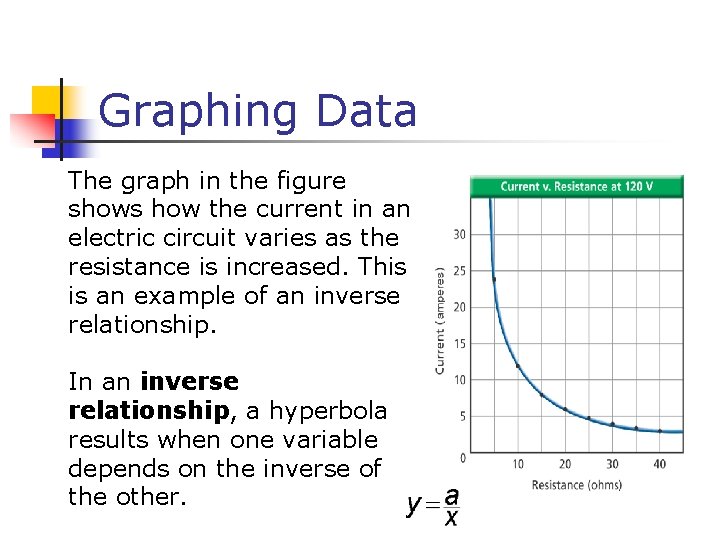
Graphing Data When the graph is not a straight line, it means that the relationship between the dependent variable and the independent variable is not linear. There are many types of nonlinear relationships in science. Two of the most common are the quadratic and inverse relationships.

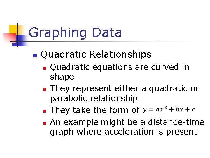
Graphing Data n Quadratic Relationships n n Quadratic equations are curved in shape They represent either a quadratic or parabolic relationship They take the form of An example might be a distance-time graph where acceleration is present

Graphing Data The graph shown in the figure is a quadratic relationship. A quadratic relationship exists when one variable depends on the square of another.

Graphing Data The graph in the figure shows how the current in an electric circuit varies as the resistance is increased. This is an example of an inverse relationship. In an inverse relationship, a hyperbola results when one variable depends on the inverse of the other.

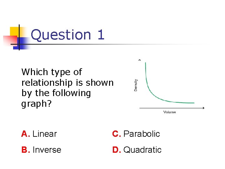
Question 1 Which type of relationship is shown by the following graph? A. Linear C. Parabolic B. Inverse D. Quadratic

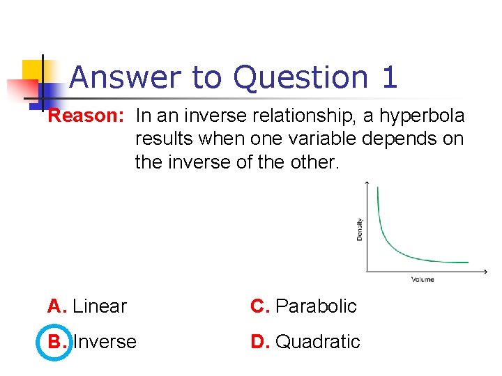
Answer to Question 1 Reason: In an inverse relationship, a hyperbola results when one variable depends on the inverse of the other. A. Linear C. Parabolic B. Inverse D. Quadratic

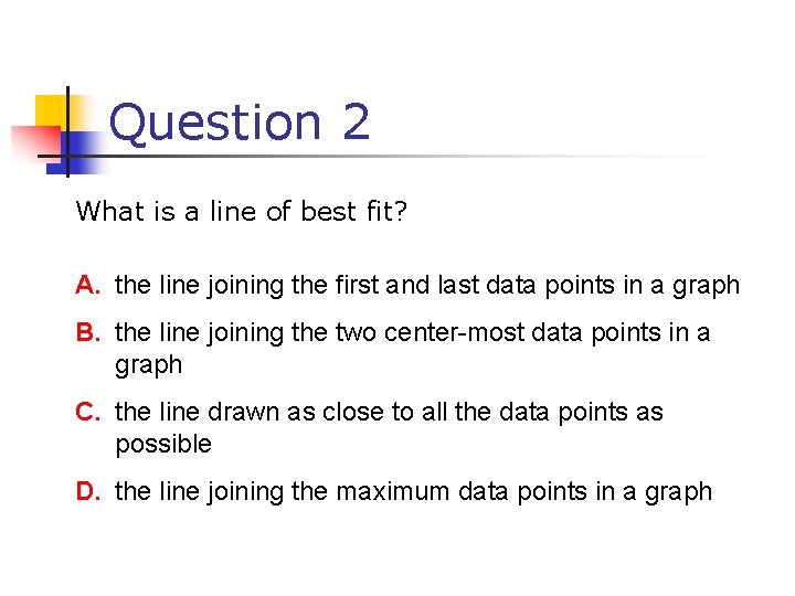
Question 2 What is a line of best fit? A. the line joining the first and last data points in a graph B. the line joining the two center-most data points in a graph C. the line drawn as close to all the data points as possible D. the line joining the maximum data points in a graph

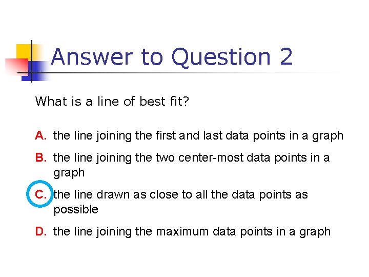
Answer to Question 2 What is a line of best fit? A. the line joining the first and last data points in a graph B. the line joining the two center-most data points in a graph C. the line drawn as close to all the data points as possible D. the line joining the maximum data points in a graph

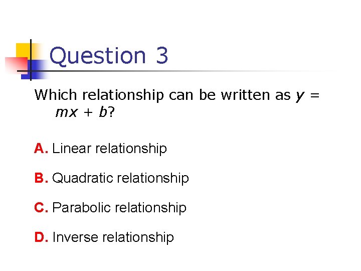
Question 3 Which relationship can be written as y = mx + b? A. Linear relationship B. Quadratic relationship C. Parabolic relationship D. Inverse relationship

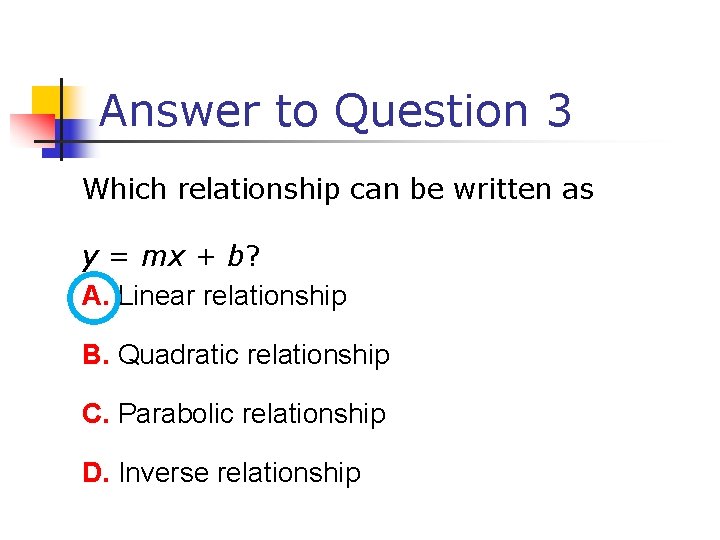
Answer to Question 3 Which relationship can be written as y = mx + b? A. Linear relationship B. Quadratic relationship C. Parabolic relationship D. Inverse relationship

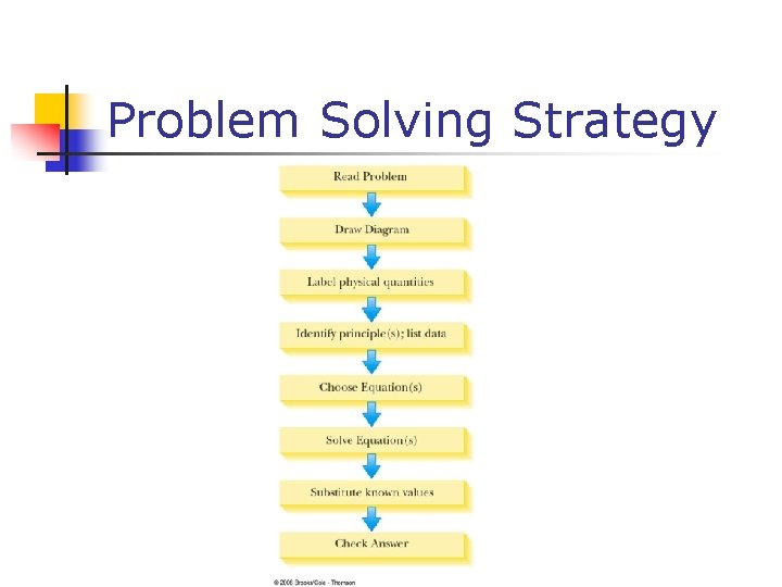
Problem Solving Strategy

Problem Solving Strategy n Read the problem n n Identify the nature of the problem Draw a diagram n Some types of problems require very specific types of diagrams

Problem Solving cont. n Label the physical quantities n n Can label on the diagram Use letters that remind you of the quantity n n n Many quantities have specific letters Choose a coordinate system and label it Identify principles and list data n n n Identify the principle involved List the data (given information) Indicate the unknown (what you are looking for)

Problem Solving, cont. n Choose equation(s) n n Based on the principle, choose an equation or set of equations to apply to the problem Substitute into the equation(s) n n Solve for the unknown quantity Substitute the data into the equation Obtain a result Include units

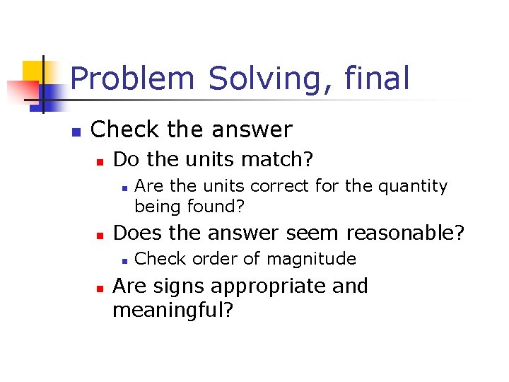
Problem Solving, final n Check the answer n Do the units match? n n Does the answer seem reasonable? n n Are the units correct for the quantity being found? Check order of magnitude Are signs appropriate and meaningful?

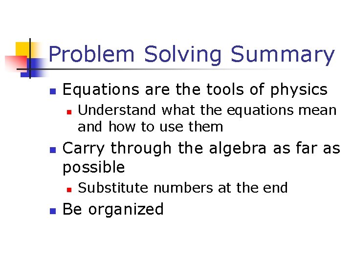
Problem Solving Summary n Equations are the tools of physics n n Carry through the algebra as far as possible n n Understand what the equations mean and how to use them Substitute numbers at the end Be organized