Physical Properties of Sea Water Property of pure

Physical Properties of Sea Water • • Property of pure water Pressure Temperature Salinity Density Equation of State Potential temperature Static Stability Reading: Talley et al. (2011): Chapter 3, S 16 Pond and Pickard (1983): Chapter 5

Pressure (p) • Pressure is the normal force per unit area exerted by water (or air in the atmosphere) on either side of the unit area. • Unit: 1 Pascal = 1 Newton/m 2 = 10 dynes/cm 2, or 1 bar = 105 Pascal = 106 dynes/cm 2. • Force due to pressure difference is down the pressure gradient. • Vertically, upward pressure gradient force is largely balanced by gravity (the hydrostatic balance). p~0 -1000 bar (A pressure change of 1 decibar (0. 1 bar) occurs over a depth change of slightly less than 1 meter). • Horizontal variation of pressure is in the order of 0. 1 bar (1 dbar) over 102 -103 kilometers, much smaller than pressure change with depth. • Accuracy of pressure measurement is 3 dbar.

Pressure and Depth Hydrostatic pressure: where d is depth (instead of height) If we choose: =1000 kg/m 3 (2 -4% lower than of sea-water) g=10 m/s 2 (2% higher than gravity) then p=1 decibar (db) is equivalent to 1 m of depth (p=1 db = 0. 1 bar = 105 dyn/cm 2 = 104 Pa (N/m 2)) • True d is 1 -2% less than the equivalent decibar depth. • A pressure change of 1 dbar occurs over a depth change of slightly less than 1 meter.

The relation between depth and pressure, using a station in the northwest Pacific at 41° 53’N, 146° 18’W. FIGURE 3. 2 TALLEY Copyright © 2011 Elsevier Inc. All rights reserved

Temperature: (T or t) • Unit: Celsius scale (o. C) in oceanography (sometimes Kelvin, K for heat content calculation, 0 o. C = 273. 16 K) • Ocean range: -1. 7 o. C (freezing point) to 30~31 o. C • Primary parameter determining density, especially in mid - and lower latitude upper ocean • Major factor in influencing the atmosphere at the surface • Temperature profile provides information on circulation features and sound speed distribution (primary parameter from surface to 500 m) • First ocean parameters to be measured and remains most widely observed

Temperature Measurement Thermometer (accuracy 0. 004 o. C, precision 0. 002 o. C) Thermistor (0. 002 o. C, 0. 0005 -0. 001 o. C) In Situ Sea Surface temperature (SST) Measurements • Bucket-sample (prior to 1950 s, thermometer) wooden to canvas (1880 -1890) bucket sampling causes cold bias of SST in 1900 s-1940 s from the level between 1850 s-1880 s (accuracy ~0. 1 o. C) • “Injection temperature” (1950 s, thermistor) measurements in the engine cooling intake water from 2 m to 5 m, partially causes a warm bias after 1940 (accuracy 0. 5 -1 o. C) • Bottles, XBTs, and CTDs • In situ observations measure “bulk” temperature (0. 5 -5 m)

Satellite SST measurement • Thermal infrared (IR) sensors (0. 5 -0. 8 K, textbook value) Scanning Radiometer (SR), 8 km resolution (early 1970 s) Advanced Very High Resolution Radiometer (AVHRR), 1 km, local precision 0. 1 o. C Cloud blocks IR totally and water vapor attenuates it (polar orbiting satellite since 1978) Atmospheric moisture correction using measurements from different channel A “blended SST analysis” combining AVHRR and in situ SST with 100 km resolution is in wide use (Reynolds 1988; Reynolds and Smith 1994, 1995), Estimated Accuracy, ± 0. 3 o. C in the tropics, ± 0. 5 o. C near the western boundary (Reynolds, 2002) • Passive microwave sensors (6 -12 GHz) Tropical Rainfall Mapping Mission (TRMM) Microwave Imager (TMI) through cloud layers lower resolution (25 -50 km) • Satellite measures the “skin layer” temperature “skin layer” is a very thin (< 1 mm) “skin” temperature is usually more than 0. 3 o colder than bulk temperature

Subsurface. Temperature Measurement Nansen bottle • Protected reversing mercury thermometer (± 0. 02 K in routine use) • in situ pressure with unprotected reversing thermometer (± 0. 5% or ± 5 m) • only a finite number (<25) of vertical points once • Deployment and retrieval typically take several hours Mechanical Bathythermograph (MBT, 1951 -1975) • Continuous temperature against depth (range, 60, 140 or 270 m) • Need calibration, T less accurate than thermometer (± 0. 2 K, ± 2 m) Expendable bathythermograph (XBT, since 1966) • Expendeble thermister casing • Accuracy, T, ± 0. 1 o. C, Z, ± 2% • dropped from moving ship of opportunity and circling aircraft • Graph of temperature against depth (resolution 65 cm) • Range of measurement: 200, 400, 800, 1500 1830 m • depth is estimated from lapsed time and known falling rate (error 20%)

Bottle measurement: An Example From Knauss: Introduction to Physical Oceanography

Expendable bathythermograph (XBT)

Heat Content of Seawater • Heat content of seawater is its thermodynamic energy • Heat content per unit volume (Joules ~ J) • T-measured temperature (K), ~ measured (derived) sea water density (kg/m 3) • cp – specific heat of sea water (dependent on temperature, salinity and pressure, determined by lab experiments, Joules/(kg K)) • Flux of heat through the surface of the volume changes heat content (if there is no source inside the volume). Heat flux per unit area per unit time has the unit of (Joules/(m 2 s))=Watts/m 2 ~ W/m 2

Heat Content cp 4. 0 X 103 J · kg-1 · °C-1 Specific heat of sea water at atmospheric pressure cp in joules per gram per degree Celsius as a function of temperature in Celsius and salinity in practical salinity units, calculated from the empirical formula given by Millero et al. , (1973) using algorithms in Fofonoff and Millard (1983). The lower line is the freezing point of salt water.

Simple Example • What surface heat flux can cause a 100 m thick layer of seawater to cool by 1 o. C in 30 days? • The total heat loss in 30 days is • Typical values of • Given values • Surface heat flux

Salinity is the total amount of dissolved material in grams in one kilogram of sea water (absolute salinity, hard to measure) Salinity is an aggregate variable. The most abundant ions in sea water: chlorine Cl- 55. 0% sodium Na+ 30. 7% sulphate SO 4++ 7. 7% magnesium Mg++ 3. 6% calcium Ca+ 1. 2% potassium K+ 1. 1% On average, there around 35 grams of salt in a kilogram of sea water, 35 g/kg, written as S=35‰ or S=35 ppt, read as “thirty-five parts per thousand” Globally, S can go from near 0 (coast) to about 40 ppt (Red Sea), BUT 90% is between 34 -35 ppt

Basic properties of salt in sea water 1). The ratio of the more abundant components remain almost constant. (ocean is very well mixed globally over geological time~millions of years, much longer than the time for water to circulate through the oceans~thousands of years) (Major exceptions are found in coastal and enclosed regions, due to land drainage and biological processes) 2). There are significant differences in total concentration of the dissolved salts from place to place and at different depths. (Processes, such as local evaporation and precipitation, as well as oceanic circulation, continually concentrate and dilute salt in sea water in specific localities) 3). The presence of salts influences most physical properties of sea water (density, compressibility, freezing point). 4). The conductivity of the sea water is partly determined by the amount of salt it contains.

Early Definition (1902) Given by a commission of the International Council for the Exploration of the Sea Total amount of solid materials in grams dissolved in one kilogram of sea water when all the carbonate has been converted to oxide, the bromine and iodine replaced by chlorine and all organic matter completely oxidized

Salinity based on chlorinity Salinity can be determined through the amount of chloride ion (plus the chlorine equivalent of the bromine and iodine), called as chlorinity, which is measured using titration with silver nitrate (Knudsen et al. , 1902) The relationship between salinity and chlorinity is based on laboratory measurements of sea water samples collected from different regions of the world ocean and was given in 1969 by UNESCO as S (‰) = 1. 80655 Chlorinity (‰) The unit of S is ppt chlorinity is the amount of chlorine ion (plus the chlorine equivalent of the bromine and iodine). Salinity is "the mass of silver required to precipitate completely the halogens in 0. 328 523 4 kg of the seawater sample. "

Practical Salinity Scale of 1978 • The practical salinity, symbol S, of a sample of sea water, is defined in terms of the ratio K 15 of the electrical conductivity of a sea water sample of 15°C and the pressure of one standard atmosphere, to that of a potassium chloride (KCl) solution, in which the mass fraction of KCl is 0. 0324356 g, at the same temperature and pressure. The K 15 value equal to one corresponds to a practical salinity equal to 35. • The corresponding formula is: S = 0. 0080 - 0. 1692 K 1/2 + 25. 3853 K + 14. 0941 K 3/2 - 7. 0261 K 2 + 2. 7081 K 5/2 +…. • Note that in this definition, S is a ratio and is non-dimensional, but salinity of 35‰ corresponds to a value of 35 in the practical salinity. • S is sometimes given the unit “psu” (practical salinity unit) in literature (probably unnecessarily) • S(ppt) = 1. 004867 S(psu)

Salinity measurement Total resolved material is hard to measure routinely in seawater (e. g. , evaporation of sea-water sample to dryness) In practice, some properties of sea water are used to estimate salinity. Method #1: Salinity is determined by measurements of a substitution quantity since it is contributed by its components in a fixed ratio. Method #2: Salinity is inferred from measurements of sea water’s electrical conductivity.

Salinity measurement Knudsen (Titration) method (precision ± 0. 02, prior to 1960) • time consuming and not convenient on board ship • not accurate enough to identify deep ocean water mass Electrical conductivity method (precision ± 0. 003~± 0. 001) • Conductivity depends on the number of dissolved ions per volume (i. e. salinity) and the mobility of the ions (ie temperature and pressure). Its units are m. S/cm (milli. Siemens per centimeter). • Conductivity increases by the same amount with S~0. 01, T~ 0. 01°C, and z~ 20 m. • The conductivity-density relation is closer than densitychlorinity • The density and conductivity is determined by the total weight of the dissolved substance

Potential temperature and temperature, (b) conductivity, and (c) salinity in the northern North Pacific. Note that conductivity is a function of temperature and pressure also, which should be compensated in the salinity measurements

Gouretski and Jancke (1995) estimated accuracy of salinity measurements as a function of time. Using high quality measurements from 16, 000 hydrographic stations in the south Atlantic from 1912 to 1991, they estimated accuracy by plotting salinity as a function of temperature using all data collected below 1500 m in twelve regions for each decade from 1920 to 1990. Standard deviation of salinity measurements at depths below 1500 m in the South Atlantic from 1920 to 1993. Each point is the average of data collected for the decade centered on the point. The value for 1995 is an estimate of the accuracy of recent measurements. From Table 1 of Gouretski and Jancke (1995).

conductivity-temperature-depth probe In situ CTD precision: S~± 0. 005 (0. 001) T ± 0. 005 K (0. 001 K) z~± 0. 15% z The vertical resolution is high T measured by thermistor S measured by conductivity cell P measured by quartz crystal CTD sensors should be calibrated (with bottle samples before 1990 s)

Absolute Salinity IOC, SCOR, and IAPSO (2010) (1) Representation of improved information about the composition of the Atlantic surface seawater used to define PSS 78 and incorporation of 2005 atomic weights (2) Corrections for the geographic dependence of the dissolved matter that is not sensed by conductivity SP: practical salinity. SR: reference salinity presently most accurate estimate of the absolute salinity of reference Atlantic surface seawater. δSA: a geographically dependent anomaly that corrects for the dissolved substances that do not affect conductivity.

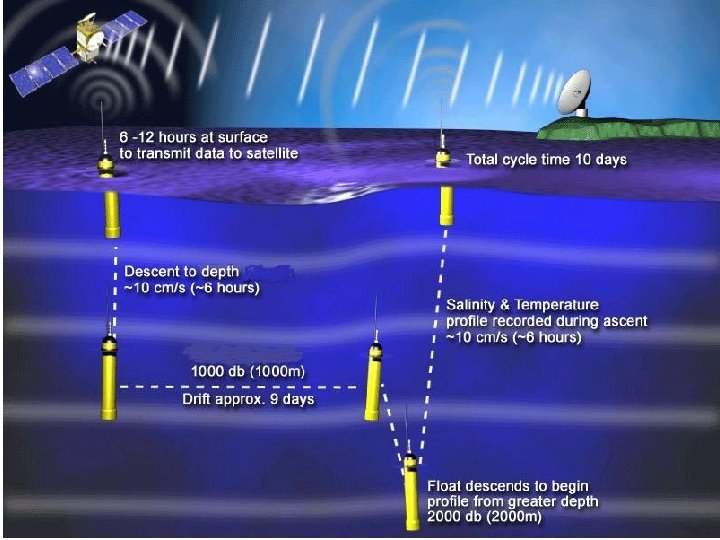
Argo Floats Modern subsurface floats remain at depth for a period of time, come to the surface briefly to transmit their data to a satellite and return to their allocated depth. These floats can therefore be programmed for any depth and can also obtain temperature and salinity data during their ascent. The most comprehensive array of such floats, known as Argo, began in the year 2000. Argo floats measure the temperature and salinity of the upper 2000 m of the ocean. This will allow continuous monitoring of the climate state of the ocean, with all data being relayed and made publicly available within hours after collection. When the Argo program is fully operational it will have 3, 000 floats in the world ocean at any one time. The accuracy of the data from the floats is 0. 005 o. C for temperature, 5 decibars for pressure, and 0. 01 for salinity (Riser et al. , 2008)

http: //www. argo. ucsd. edu/About_Argo. html An Argo profile from the subtropical North Pacific (20. 25 N 121. 4 W, May 15 2004)

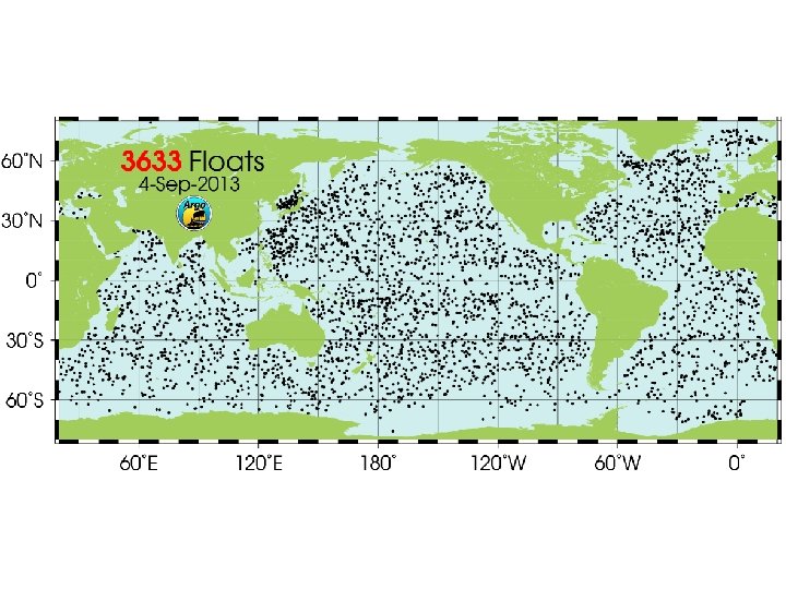
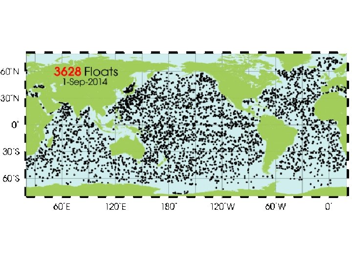
Positions of the floats that have delivered data within the last 30 days http: //www. argo. ucsd. edu

Summary of Measurement Accuracy Variable Range Best Accuracy Temperature Salinity 42°C Pressure Density Equation of State 10, 000 dbar ± 0. 001°C ± 0. 02 by titration ± 0. 005 by conductivity ± 0. 65 dbar ± 0. 005 kg/m 3 ± 0. 009 kg/m 3 Quality Controlled in situ ocean temperature and salinity profiles database: As of 2008: ~one million XBT profiles ~700, 000 CTD profiles ~60, 000 Argo profiles ~1, 100, 000 Nansen bottle data

Density ( , kg/m 3) • Determine the depth a water mass settles in equilibrium. • Determine the large scale circulation. • changes in the ocean is small. 1021 -1070 kg/m 3 (depth 0~10, 000 m) • increases with p (the greatest effect) ignoring p effect: ~1020. 0 -1030. 0 kg/m 3 1027. 7 -1027. 9 kg/m 3 for 50% of ocean • increases with increasing S. decreases with increasing T most of the time. • is usually not directly measured but determined from T, S, and p

FIGURE 3. 4 Increase in density with pressure for a water parcel of temperature 0°C and salinity 35. 0 at the sea surface. TALLEY Copyright © 2011 Elsevier Inc. All rights reserved

Density anomaly Since the first two digits of never change, a new quantity is defined as s, t, p = – 1000 kg/m 3 called as “in-situ density anomaly”. (1000 kg/m 3 is for freshwater at 4 o. C) Atmospheric-pressure density anomaly (Sigma-tee) t = s, t, 0 – 1000 kg/m (note: s and t are in situ at the depth of measurement)

Equation of State The dependence of density (or ) on temperature T, salinity S and pressure p is the Equation of State of Sea Water. Bulk modulus K=1/ , is compressibility. , C speed of the sound in sea water. = (T, S, p) is determined by laboratory experiments. International Equation of State (1980) is the most widely used density formula now. • This equation uses T in °C, S from the Practical Salinity Scale and p in dbar (1 dbar = 104 Pascal = 104 N m-2) and gives in kg m 3. • Range: -2 o. C≤ T ≤ 40 o. C, 0 ≤ S ≤ 40, 0 ≤ p ≤ 105 k. Pa (depth, 0 to 10, 000 m) • Accuracy: 5 x 10 -6 (relative to pure water, ± 0. 005) • Polynomial expressions of (S, t, 0) (15 terms) and K(S, t, p) (27 terms) get accuracy of 9 x 10 -6.

FIGURE 3. 1 Values of density t (curved lines) and the loci of maximum density and freezing point (at atmospheric pressure) for seawater as functions of temperature and salinity. The full density is 1000 + t with units of kg/m 3. TALLEY Copyright © 2011 Elsevier Inc. All rights reserved

Relation between (T, S) and t t as a function of T and S • The relation is more nonlinear with respect to T • t change is more uniform with S • t is more sensitive to S than T near freezing point • max meets the freezing point at S =24. 7 S < 24. 7: after passing max surface water becomes lighter and eventually freezes over if cooled further. The deep basins are filled with water of maximum density The temperature of density maximum is the red line and the freezing point is the light blue line S > 24. 7: Convection always reaches the entire water body. Cooling is slowed down because a large amount of heat is stored in the water body

Simple formula: (1) accuracy: ± 0. 5 kg/m 3 where 0=1027 kg/m 3, T 0=10 o. C, S 0=35 psu, a=-0. 15 kg/m 3 o. C, b=0. 78 kg/m 3, k=4. 5 x 10 -3 /dbar (2) where For 30≤S≤ 40, -2≤T≤ 30, p≤ 6 km, good to 0. 16 kg/m 3 For 0 ≤S≤ 40, good to 0. 3 kg/m 3

Potential density relative to (a) 0 dbar and (b) 4000 dbar as a function of potential temperature (relative to 0 dbar) and salinity. Parcels labeled 1 have the same density at the sea surface. The parcels labeled 2 represents Mediterranean (saltier) and Nordic Seas (fresher) source waters at their sills. FIGURE 3. 5 TALLEY Copyright © 2011 Elsevier Inc. All rights reserved

Thermobaricity: cold water is more compressible than warm water http: //www. oc. nps. edu/thermobaricity/thermobanim. html

Mixing in the Ocean: Cabelling

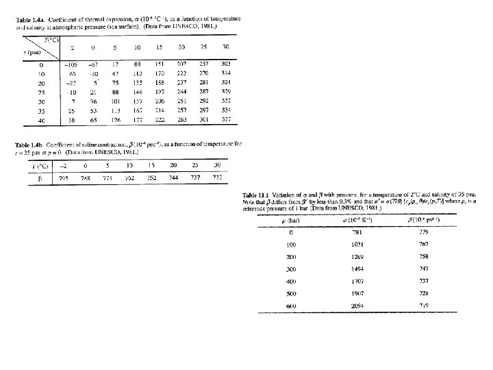
Specific volume and anomaly Specific volume: =1/ (unit m 3/kg) Specific volume anomaly: = s, t, p – 35, 0, p (usually positive) • = s + t + s, p + t, p + s, t, p • In practice, s, t, p is always small (ignored) • s, p and t, p are smaller than the first three terms (5 to 15 x 10 -8 m 3/kg per 1000 m) Thermosteric anomaly: S, T = s + t + s, t (50 -100 x 10 -8 m 3/kg or 50 -100 centiliter per ton, c. L/t)

Converting formula for S, T and t : Since (35, 0, 0)=0. 97266 x 10 -3 m 3/kg, , m 3/kg For 23 ≤ t ≤ 28, , accurate to 0. 1 accurate to 1 in c. L/ton For most part of the ocean, 25. 5 ≤ t≤ 28. 5. Correspondingly, 250 c. L/ton ≥ S, T ≥ -50 c. L/ton