Physical Modeling Time Lapse 3 D and VSP

Physical Modeling: Time Lapse, 3 D, and VSP Robert W. Wiley Allied Geophysical Laboratories University of Houston

Outline • • Properties of Physical Modeling Fracture Model Time-Lapse Model 3 D VSP Model Hardware Future Directions Conclusions

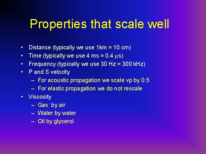
Properties that scale well • • Distance (typically we use 1 km = 10 cm) Time (typically we use 4 ms = 0. 4 s) Frequency (typically we use 30 Hz = 300 k. Hz) P and S velocity – For acoustic propagation we scale vp by 0. 5 – For elastic propagation we do not rescale • Viscosity – Gas by air – Water by water – Oil by glycerol

Properties that do not scale well • Source and receiver size • Pore size (other physics takes place for extremely small pores) • Frequency dependent attenuation mechanisms (which we don’t yet understand anyway!) • Soft sediments and weathering zones Other limitations • A model 1 m by 0. 5 m (corresponding to 10 km x 10 km by 5 km) weighs more than one metric ton! • Models take months to build • We needed bigger, stronger, and more patient graduate students!

Fracture Model

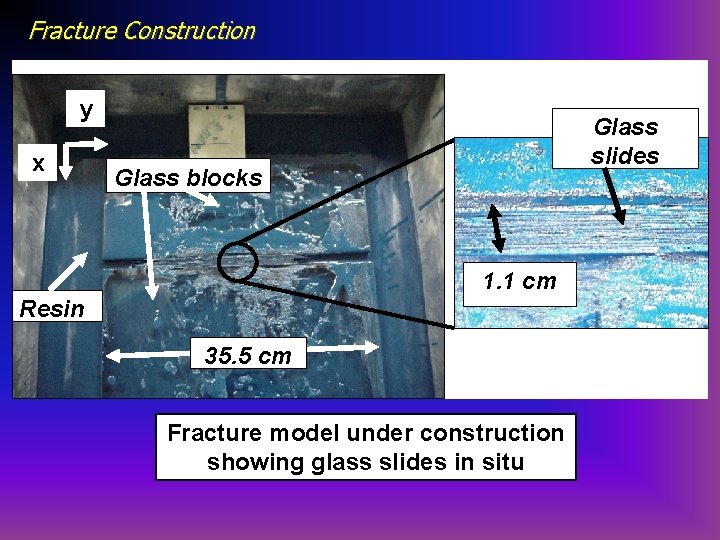
Fracture Construction y x Glass slides Glass blocks 1. 1 cm Resin 35. 5 cm Fracture model under construction showing glass slides in situ

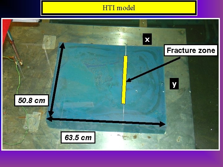
HTI model x Fracture zone y 50. 8 cm 63. 5 cm

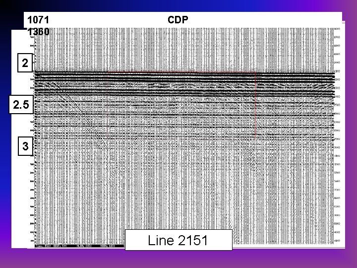
1071 1360 CDP 2 2. 5 3 Line 2151

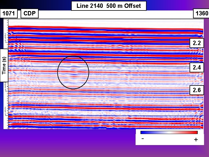
Line 2140 500 m Offset 1071 CDP 1360 Time (s) 2. 2 2. 4 2. 6 + -

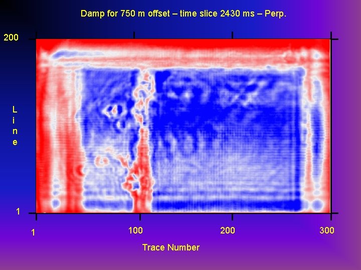
Damp for 750 m offset – time slice 2430 ms – Perp. 200 L i n e 1 1 100 Trace Number 200 300

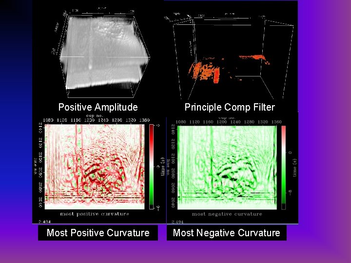
Positive Amplitude Principle Comp Filter Most Positive Curvature Most Negative Curvature

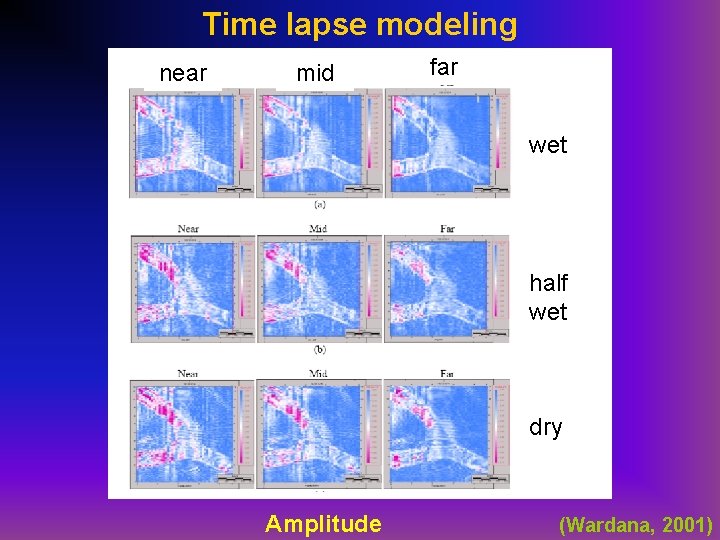
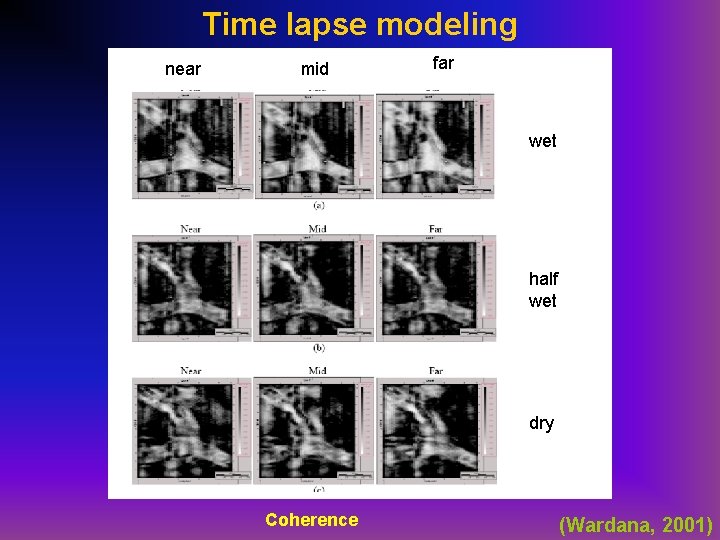
Time-Lapse Model

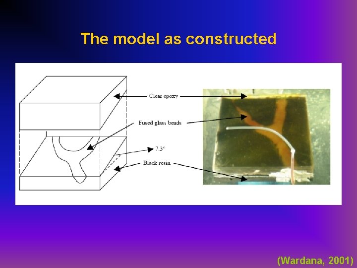
The model as constructed (Wardana, 2001)

Time lapse modeling near mid far wet half wet dry Amplitude (Wardana, 2001)

Time lapse modeling near mid far wet half wet dry Coherence (Wardana, 2001)

3 D VSP Model

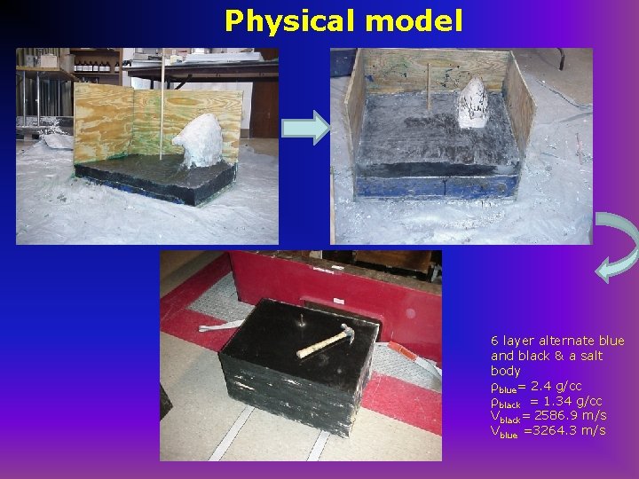
Physical model 6 layer alternate blue and black & a salt body ρblue= 2. 4 g/cc ρblack = 1. 34 g/cc Vblack= 2586. 9 m/s Vblue =3264. 3 m/s

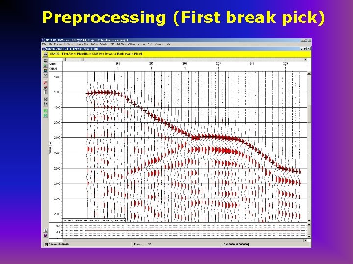
Preprocessing (First break pick)

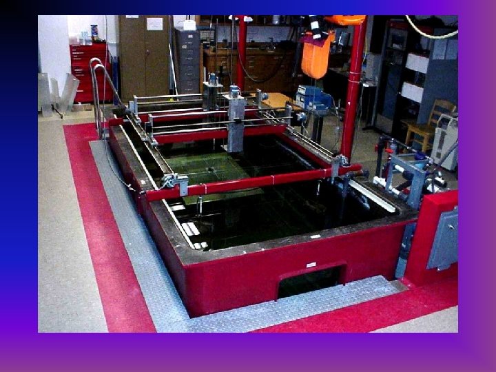
Hardware

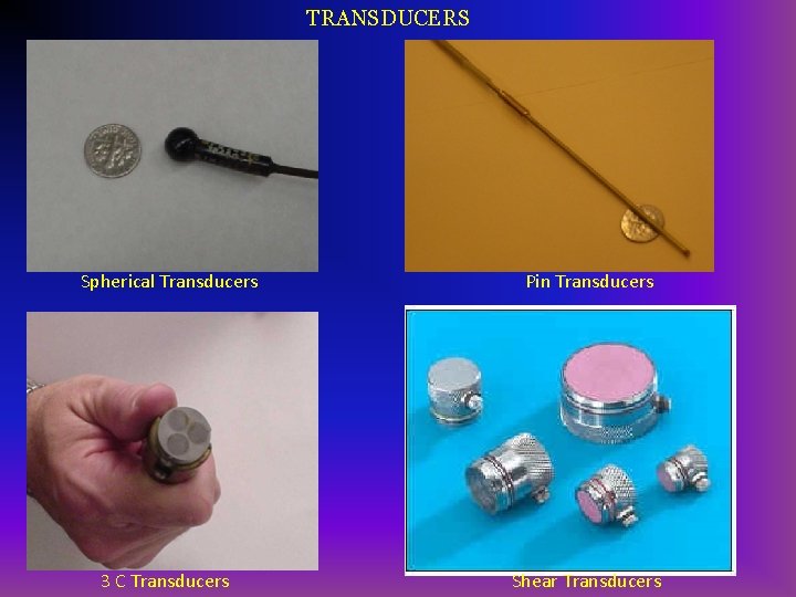
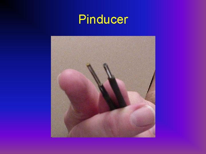
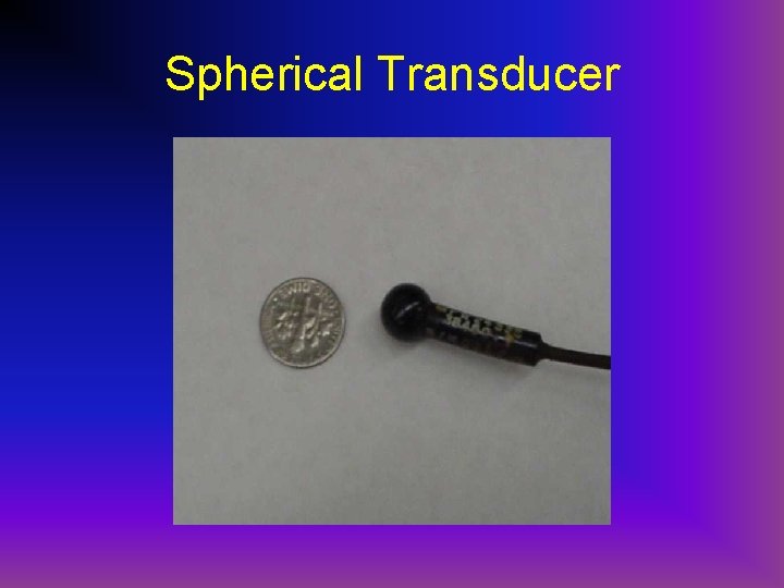
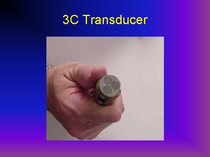
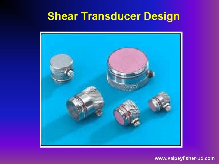
TRANSDUCERS Spherical Transducers Pin Transducers 3 C Transducers Shear Transducers

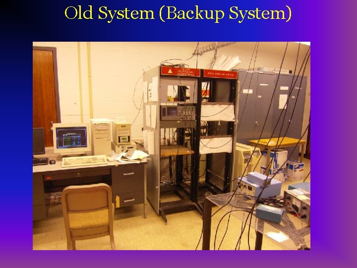
Old System (Backup System)

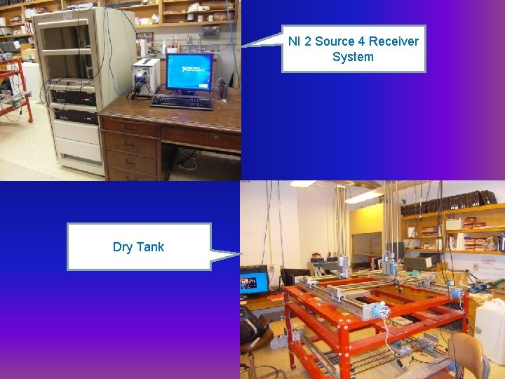
NI 2 Source 4 Receiver System Dry Tank

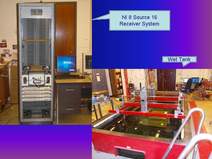
NI 8 Source 16 Receiver System Wet Tank

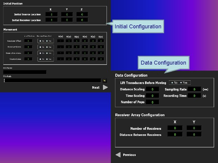
Initial Configuration Data Configuration

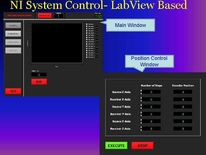
NI System Control- Lab. View Based Main Window Position Control Window

Future Directions • • • Bring the two new systems on line Develop a 16 receiver system Develop a multiple source system Collect porous model data Test additional transducers Investigate other materials

Conclusions • We are able to build reasonably complex physical models • Results are similar to seismic data • This is an excellent approach to acquiring controlled data for testing algorithms • Physical modeling is cost effective compared to field experiments

Thank You

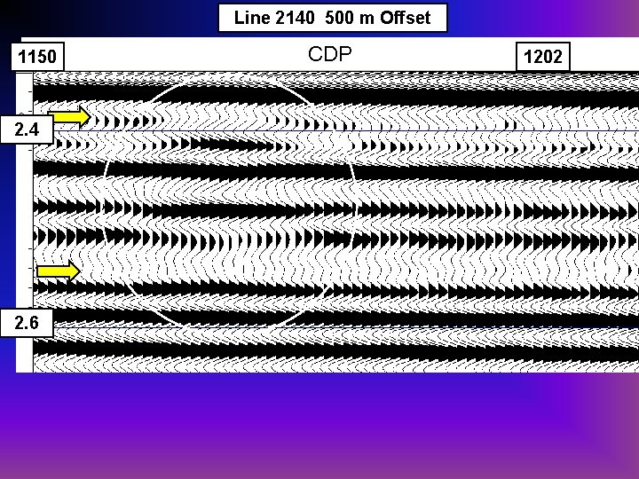
Line 2140 500 m Offset 1150 2. 4 2. 6 CDP Curvature 1202

Pinducer

Physical Limitations • Inaccurate construction of actual model • Limited selection of velocity and density parameters

Some Limitations • Limited bandwidth with strong resonance at one frequency • Limited to materials with specific elastic parameters • Difficult to build lateral velocity variations • Labor intensive • Cannot model all real earth materials/layers

Source and Receiver Issues • Inaccurate location of source and receiver with respect to the model • Source and receiver resonate at one frequency • Source and receiver dimensions are large • Source and receiver have pronounced radiation patterns

Line 2140 500 m Offset 1071 CDP 1360 Time (s) 2. 2 2. 4 2. 6 + -

Properties that do not scale well • Source and receiver size • Pore size (other physics takes place for extremely small pores) • Frequency dependent attenuation mechanisms (which we don’t yet understand anyway!) • Soft sediments and weathering zones Other limitations • A model 1 m by 0. 5 m (corresponding to 10 km x 10 km by 5 km) weighs more than one metric ton! • Models take months to build • We needed bigger, stronger, and more patient graduate students!

Why Run Models • To test interpretation – Salt dome, coal seam • To test algorithm – Migration, Multiple removal • To test interpretation tools – fracture identification, fluid content • To test theory – Lamb’s problem, Kirchhoff diffraction, anisotropy

Why Physical Modeling • No simplifying mathematical assumptions • No approximations to mathematical functions • No round-off errors • No a priori mathematical understanding required

Limitations • Limited selection of velocity and density parameters • Difficult to build lateral velocity variations • Labor intensive • Inaccurate construction of actual model • Limited to frequency response of transducers • Source and receiver dimensions

Benefits of Physical Modeling • Experimental repeatability and controlled conditions • Very cost-effective compared to field work • Physics of elastic energy propagation through physical models is same as real world • Arbitrary earthlike conditions closer to real earth data than numerical modeling

Spherical Transducer

3 C Transducer

Shear Transducer Design www. valpeyfisher-ud. com