Physical and Dynamical Oceanography CLIM 712 Class 12

Physical and Dynamical Oceanography CLIM 712 Class: 12: 00 pm – 1: 15 pm, Tuesday, Thursday (Research Hall 201) Office hour: 9: 00 am – 10: 30 am, Tuesday (Research Hall, 269) Bohua Huang Department of Atmospheric, Oceanic, and Earth Sciences College of Science George Mason University Center for Ocean-Land-Atmosphere Studies Phone: 703 -993 -6084 Email: huangb@cola. iges. org bhuang@gmu. edu

References Text books: • Pond, S. , and G. L. Pickard, 1983: Introductory Dynamical Oceanography. 2 nd edition, 329 pp, Butterworth-Heinemann. • Talley, L. D. , Pickard, G. L. , W. J. Emery, J. H. Swift, 2011: Descriptive Physical Oceanography, 6 th edition, 555 pp, ELSEVIER. Other titles of interest: • Pickard, G. L. , and W. J. Emery, 1993: Descriptive Physical Oceanography, 5 th enlarged edition, 320 pp, Pergamon Press. • Mellor, G. L. , 1996: Introduction to Physical Oceanography, 260 pp, AIP Press. • Knauss, J. A. , 1997: Introduction to Physical Oceanography, 309 pp, 2 nd edition, Prentice-Hall. • Pedlosky, J. , 1987: Geophysical Fluid Dynamics, 710 pp, Springer-Verlag • Mc. Williams, J. C. , 2006: Fundamentals of Geophysical Fluid Dynamics, 249 pp, Cambridge. More advanced readings: • Abarbanel, H. D. I. , and W. R. Young, Eds. , 1987: General Circulation of the Ocean, 291 pp. Springer-Verlag. • Pedlosky, J. , 1996: Ocean Circulation Theory, 453 pp, Springer. • Siedler, G. , J. Church, and J. Gould, Eds. , 2001: Ocean Circulation and Climate, 715 pp. , Academic Press. • Pedlosky, J. , 2003: Waves in the Ocean and Atmosphere, 260 pp, Springer-Verlag. • van Aken, H. M. , 2006: The Oceanic Thermohaline Circulation, An Introduction. 326 pp, Springer

Useful Online Physical Oceanography Books • R. H. Stewart: Introduction to Physical Oceanography (http: //oceanworld. tamu. edu/resources/ocng_textbook/contents. html) • M. Tomczak: Introduction to Physical Oceanography (http: //gaea. es. flinders. edu. au/~mattom/Intro. Oc/newstart. html) • M. Tomczak, & J. S. Godfrey: Regional Oceanography: an Introduction (http: //gaea. es. flinders. edu. au/~mattom/regoc/index. html) B. A. Warren & C. Wunsch (Ed. , ): Evolution of Physical Oceanography (http: //ocw. mit. edu/ans 7870/resources/Wunsch/wunschtext. htm )

Requirement • Homework: 5 assignments (every other week since Week 3, 50%) • Mid-term exam (Oct 16, close book, 20%) • Final exam (Dec 11, 10: 30 am-1: 15 pm, open book, 20%) • Term paper (topics in NOAA monthly ocean briefing, research paper style, 4 pages, double space, 10%) Slides of the lectures will be on: ftp: //cola. gmu. edu/pub/huangb/Fall 14 before each class

Major Topics • Properties of seawater • Heat, freshwater and momentum fluxes and conservation laws • Global T-S distribution • Fluid dynamics on rotating sphere • Description of large-scale gyres • Barotropic dynamics of large-scale gyres • Mixing, turbulence, surface layer • Large-scale overturning and thermohaline circulation • Rossby waves, instability and mesoscale eddies • Surface gravity waves (nonrotating and rotating) • Internal gravity waves • Tides • Coastal processes: currents, fronts, estuaries • Air-sea interaction: El Niño

Course Outline [Numbers in brackets give chapters to read in Descriptive Physical Oceanography, 6 th Ed. (Des), and Introductory Dynamical Oceanography, 2 nd Ed. (Dyn). Lectures do not cover the entirety of all chapters assigned; students will only be responsible for material covered in lectures. For some topics, additional reading materials will be supplied with class notes] • Properties of seawater [Des 2, 3] – – – • Global T-S distribution [Des 4 ] – – • Coriolis force equations of motion geostrophy Ekman layers Description of large-scale gyres [Des 7, 9, 10] – – • heat flux components heat flux distribution evaporation, precipitation, runoff box models Momentum flux, surface wind stress Fluid dynamics on rotating sphere [Des 7, Dyn 6, 8, 9. 1 -9. 4] – – • surface profiles vertical profiles static stability annual cycle and interannual variability T-S Forcing and conservation laws [Des 5] – – – • composition equation of state measurement: T, S, pressure wind patterns and gyres western and eastern boundary currents polar currents equatorial currents Barotropic dynamics of large-scale gyres [Dyn 9. 5 -9. 14] – – – vorticity dynamics gyres and western boundary currents Sverdrup, Stommel, and Munk

• • Mixing, turbulence, surface layer [supplied reading] - descriptive Kelvin-Helmholtz instability - surface mixed layer dynamics - sources of subsurface mixing Large-scale overturning [Des 14, supplied reading] - thermohaline structure and meridional overturning - advective-diffusive balance and overturning - Stommel-Arons patterns - subduction and shallow cells Surface gravity waves (nonrotating and rotating) [Dyn 12. 1 -12. 8, 12. 10. 1 -12. 10. 3] - short and long nonrotating SGWs - Poincare and Kelvin waves Tides [Des 8, Dyn 13. 1 -13. 7] - tidal forcing - equilibrium theory - forced response Internal gravity waves [Dyn 12. 9] - two-layer fluid - rotational effects - continuous fluid Rossby waves, instability and mesoscale eddies [supplied reading] - Rossby wave dynamics - observations of eddies Coastal processes: currents, fronts, estuaries [Des 8] El Nino [supplied reading] - air-sea feedbacks - equatorial waveguide - ENSO description

Introduction What is Physical Oceanography? Why is ocean important for climate? How do we do it? A brief history of physical oceanography Reading: Talley et al. Chapter 1 and S 1

What is Physical Oceanography? A knowledge of the circulation of the oceans; a systematic quantitative description of the character of the ocean waters and of their movements 1). A description of the temperature, salinity, and density patterns in the ocean, including their variability. 2). The three dimensional water movement (the circulation: currents and vertical movements; also, waves and tides). 3). The transfer of mass, energy, and momentum between the ocean and the atmosphere. 4). The mechanisms of these properties and processes. Simply: • What temperature is the water? • What salinity is the water? • Where is the water going? • Why is that? Understanding large-scale, nearly horizontal, nearly frictionless fluid ocean behaves based on observations of the circulation and water properties

FIGURE 1. 2 Time and space scales of physical oceanographic phenomena from bubbles and capillary waves to changes in ocean circulation associated with Earth’s orbit variations. TALLEY Copyright © 2011 Elsevier Inc. All rights reserved

Why is ocean important for climate? Ocean is a major component of the earth climate system

Ocean plays important roles in maintaining the earth climate • Ocean has large heat storage -Roughly, 3 meters of sea water has about the same heat capacity as the whole atmospheric column above it -Ocean heat storage modulates diurnal and seasonal cycles and climate variations -Maritime climate is generally milder than continental climate

• Ocean transfers heat and freshwater over a wide range of time and space scales -- The earth system is not in local radiative heat balance -- The tropics gaining and the polar regions losing heat -- Meridional oceanic heat transport is comparable to that of the atmosphere

Fluctuations within the ocean affect the climate significantly. Sea surface temperature (SST) changes from year-toyear significantly. The SST anomalies can persist for a long time.

The SST anomalies have serious consequences to the weather and climate

Air-sea interaction is an important source for global climate variability (e. g. , ENSO) Ocean provides the “memory” of the low frequency fluctuations

Global SST Anomaly (0 C) and Anomaly Tendency (from CPC) - Negative SSTA presented in the tropical eastern and central Pacific, consistent with La Niña conditions. - Negative PDO SST pattern presented in N. Pacific. - Positive SSTA presented in the tropical Indian Ocean and tropical W. Pacific. - Tripole SST anomaly pattern persisted in North Atlantic, and positive SSTA in the tropical North Atlantic has been near historical high during Mar-Jul 2010. - SSTA continuously decreased in the central and eastern tropical Pacific, suggesting strengthening of La Niña conditions. - SST tendency was large in N. Pacific. - Both positive and negative SST tendency existed in the tropical Indian Ocean. - Tripole SSTA tendency pattern suggested the persistency and slightly northward shift of the tripole SSTA pattern in North Atlantic. Fig. G 1. Sea surface temperature anomalies (top) and anomaly tendency (bottom). Data are derived from the NCEP OI SST analysis, and anomalies are departures from the 1971 -2000 base period means.

Global SST Anomaly (0 C) and Anomaly Tendency - Neutral SSTA persisted over the equatorial Pacific Ocean. - A horseshoe pattern in the North Pacific intensified. - Negative SSTA prevailed over the extratropical North Atlantic and SST in the tropical Atlantic was above normal. - Positive SSTA was observed in mid -latitude southern oceans. - Minor tendencies presented in the central and eastern tropical Pacific. - The horseshoe pattern of North Pacific further intensified in Jul 2011. - Small positive and large negative tendencies were observed in the North Atlantic. Fig. G 1. Sea surface temperature anomalies (top) and anomaly tendency (bottom). Data are derived from the NCEP OI SST analysis, and anomalies are departures from the 1971 -2000 base period means.

Global SST Anomaly (0 C) and Anomaly Tendency - Positive SST anomalies presented in the central-eastern equatorial Pacific. - Large positive SST anomalies presented in the Artic Ocean, subpolar North Atlantic, and along the Gulf Stream. - Negative PDO-like pattern presented in North Pacific. - Negative(positive) SST anomalies presented north of Australia (in southeast subtropical Indian Ocean). - A weak warming tendency presented in the central-eastern equatorial Pacific. - A strong warming tendency presented in the Artic Ocean, subpolar North Atlantic and the western-central North Pacific. Fig. G 1. Sea surface temperature anomalies (top) and anomaly tendency (bottom). Data are derived from the NCEP OI SST analysis, and anomalies are departures from the 1981 -2010 base period means.

Global SST Anomaly (0 C) and Anomaly Tendency - SST was near-normal across the western -central tropical Pacific and below average across the eastern Pacific. - Strong positive SST anomalies were observed in the high latitudes of North Pacific, North Atlantic, and Arctic Oceans. - A strong warming tendency was observed in the high latitudes of North Pacific, North Atlantic and Artic Oceans. Fig. G 1. Sea surface temperature anomalies (top) and anomaly tendency (bottom). Data are derived from the NCEP OI SST analysis, and anomalies are departures from the 1981 -2010 base period means.

Global SST Anomaly (0 C) and Anomaly Tendency - Large positive SSTA presented in the high-latitude of North Pacific and the Arctic Ocean - Strong warming continued in the Norwegian Sea. - SST were above-average in the equatorial eastern Pacific Ocean. - Positive SSTA dominated in the South Ocean. - Negative SSTA tendencies were observed across the equatorial Pacific and Atlantic Oceans. - A strong warming presented in the western North Atlantic. - A tripolar tendency pattern presented in the North Pacific Ocean. Fig. G 1. Sea surface temperature anomalies (top) and anomaly tendency (bottom). Data are derived from the NCEP OI SST analysis, and anomalies are departures from the 1981 -2010 base period means.

Atlantic Multidecadal Oscillation

Figure 5. 1. Time series of global annual ocean heat content (1022 J) for the 0 to 700 m layer. The black curve is updated from Levitus et al. (2005), with the shading representing the 90% confidence interval. The red and green curves are updates of the analyses by Ishii et al. (2006) and Willis et al. (2004, over 0 to 750 m) respectively, with the error bars denoting the 90% confidence interval. The black and red curves denote the deviation from the 1961 to 1990 average and the shorter green curve denotes the deviation from the average of the black curve for the period 1993 to 2003 (IPCC Report).

Global ocean circulation may be changed fundamentally by climate change And the oceanic circulation change will feedback seriously to the earth climate.

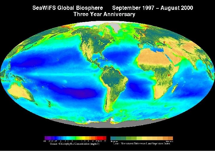
ocean circulation and marine biology -- T and S distribution affects phytoplankton -- Current affects the concentration and dispersion -- Mixing and upwelling are important to provide nutrients -- Phytoplankton changes the ocean color -- Phytoplankton represents the first link in the marine food web -- Phytoplankton has a major role in the global carbon cycle -- An indicator of circulation change -- Biological feedback to circulation?

Ocean Color and El Niño As indicated by the red (warm) region off the west coast of Peru (top image), El Niño was still going strong in February 1998. Phytoplankton were growing just to the north of the equator (bright blue green region in the image second from top). By February 1999 La Niña had replaced El Niño, and the equatorial Pacific had strong phytoplankton production (bottom pair of images). Images by Robert Simmon based on data from the Distributed Active Archive Centers at the JPL and GSFC

Knowledge of ocean circulation, especially coastal processes, is helpful for environmental sciences -- pollution -- oil drilling -- oil spills -- sewage outfalls -- industrial waste

How do we do it? The approach of physical oceanography research • observations to get the basic phenomenon • applying laws of physics to explain the features we find (hypothesis/theory) • theory leads us to find new information to verify its predictions (more observation) • new observations test (verify, modify, or disprove) theory (improved theory) • general circulation models blurs the boundary between traditional physical and dynamical branches

Figure 1. 1 Data, numerical models, and theory are all necessary to understand the ocean. Eventually, an understanding of the ocean-atmosphere-land system will lead to predictions of future states of the system (From Stuart 2007).

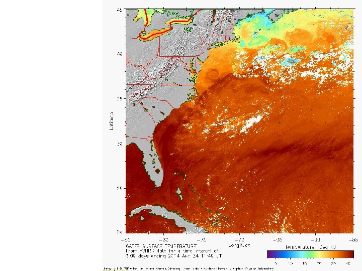
Gulf Stream An Example Narrow, has a width of 100 km Warm core, carries subtropical water northward Large meanders and rings (mesoscale eddy) Permanent, part of a large-scale gyre circulation (gyre scale ~103 km)

Questions: Why does the Gulf Stream concentrate near the western boundary? What determines its width and speed? Why are there meanders and rings? Any climate significance? …….

(b) Franklin-Folger map of the Gulf Stream. Source: From Richardson (1980 a). FIGURE 1. 1 b TALLEY Copyright © 2011 Elsevier Inc. All rights reserved

A Brief History of Oceanographic Exploration Surface Oceanography- major approach prior to 1873 Systematic collection of phenomena observable from the deck of sailing ships (marine winds, currents, waves, temperature etc. ) Examples: Halley’s charts of the trade-winds (1685); Hadley(1735) Franklin’s map of the Gulf Stream (1769) Maury's Physical Geography for the Sea (1847) Pillsbury's measurements of the Florida Current (1885)

Oceanographic Expeditions Wide range survey of surface and subsurface oceanic conditions Examples: Challenger Expedition (British, 1872 -1876) Main interest in marine life below 600 m but also collected large amount of physical measurements in the Atlantic and Pacific Fram Expedition (Norway, 1895 -1896) Leaded by Nansen, polar sea exploration Meteor Expedition (German, 1925 -1927) Leaded first by Merz and later by Wüst, concentrated on overturning circulation. The ship travels 67, 000 miles, made 14 sections across the Atlantic, 310 hydrographic stations, 33, 000 depth sounding Other Acchivements The Scandinavian Scientists developed the “dynamical method” to derive geostropic currents from T-S observations Reversing thermometer gives more accurate subsurface temperature measurements

Upper panel: Track of the H. M. S. Challanger during the British Challanger Expedition 1872 -1876. From Wüst (1964). Right panel: Track of the R/V Meteor during the German Meteor Expedition. From Wüst (1964).

International Programs: 1957 -1978 • Multi-national surveys of oceans and studies of oceanic processes. Example: International Geophysical Year cruises • Multiship studies of oceanic processes: e. g. , MODE, POLYMODE experiments • New Technologies improve observations significantly Bruce Hamon and Neil Brown develop the CTD for measuring conductivity and temperature as a function of depth in the ocean (1955). Sippican Corporation (Tim Francis, William Van Allen Clark, Graham Campbell, and Sam Francis) invents the Expendable Bathy Thermograph (XBT), now perhaps the most widely used oceanographic instrument (1963).

The sections in the International Geophysical Year Atlantic Program 1957 -1959. From Wüst (1964).

Satellite Remote Sensing (since 1978) Global surveys of oceanic processes from space Examples Seasat (1978) NOAA 6 -17 (1979 -2002) NIMBUS-7 (1978 -1994) Geosat (1985 -1990) Topex/Poseidon (1992 -) ERS 1 & 2(1991 -00, 1995) Topex/Poseidon tracks in the Pacific Ocean during a 10 -day repeat of the orbit. From Topex/Poseidon Project.

Earth System Study Global studies of the interaction of biological, chemical, and physical processes in the ocean, the atmosphere and the land using in situ and space data as well as coupled models. Oceanic examples Tropical Ocean-Global Atmosphere (TOGA) Program (1985 -1995) World Ocean Circulation Experiment (WOCE, 1991 -1996) Joint Global Ocean Flux Study (JGOFS)

World Ocean Circulation Experiment: Tracks of research ships making a one-time global survey of the oceans of the world

Some Theoretical Milestones • 1775 Laplace's published his theory of tides. • 1800 Rumford proposed a meridional circulation of the ocean with water sinking near the poles and rising near the Equator. • 1905 Ekman published his paper on wind-driven oceanic boundary layer. • 1910 -1913 Vilhelm Bjerknes published Dynamic Meteorology and Hydrography which laid the foundation of geophysical fluid dynamics. • 1942 Publication of The Oceans by Sverdrup, Johnson, and Fleming, the first comprehensive survey of oceanographic knowledge. • 1947 -1950 Sverdrup, Stommel, and Munk publish their theories of the winddriven circulation of the ocean. Together the three papers lay the foundation for our understanding of the ocean's circulation. • 1958 Stommel publishes his theory for the deep circulation of the ocean. • 1969 Kirk Bryan and Michael Cox develop the first numerical model of the oceanic circulation. • ……