Phylogenetic Trees Lecture 13 NOTE THE PDF FORMAT

Phylogenetic Trees Lecture 13 NOTE: THE PDF FORMAT INCLUDES MORE SLIDES Background reading: Durbin et al Chapter 8. . This class consists of parts of Prof Joe Felsenstein’s lectures 4 and 5 taken from: http: //evolution. genetics. washington. edu/genet 541/2002/lecture 5. pdf and on Chapter 8. 2 of Durbin et al. Edited by Dan Geiger.

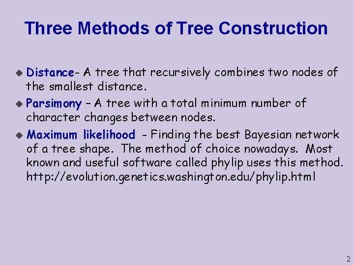
Three Methods of Tree Construction Distance- A tree that recursively combines two nodes of the smallest distance. u Parsimony – A tree with a total minimum number of character changes between nodes. u Maximum likelihood - Finding the best Bayesian network of a tree shape. The method of choice nowadays. Most known and useful software called phylip uses this method. http: //evolution. genetics. washington. edu/phylip. html u 2

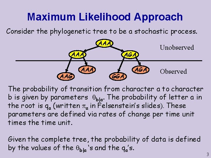
Maximum Likelihood Approach Consider the phylogenetic tree to be a stochastic process. AAA AAG AAA AGA GGA AGA Unobserved Observed The probability of transition from character a to character b is given by parameters b|a. The probability of letter a in the root is qa (written a in Felsenstein’s slides). These parameters are defined via rates of change per time unit times the time unit. Given the complete tree, the probability of data is defined by the values of the b|a ‘s and the qa’s. 3

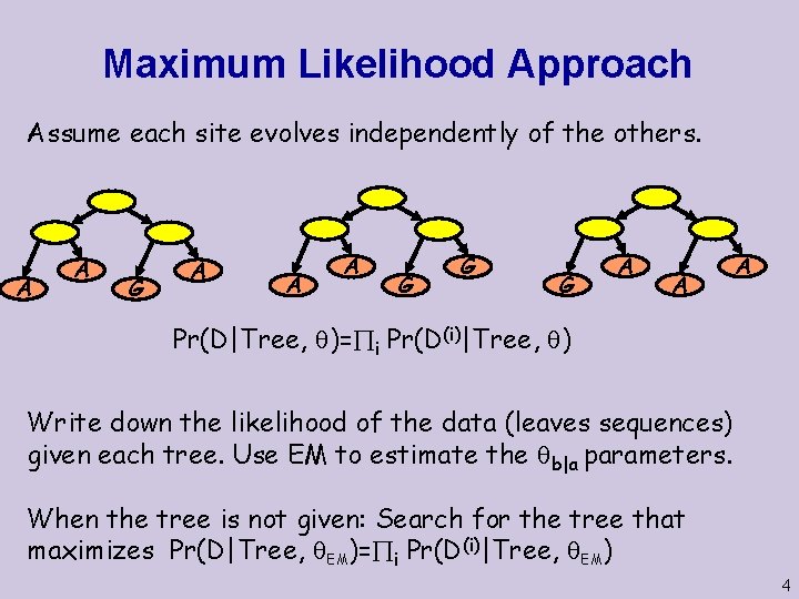
Maximum Likelihood Approach Assume each site evolves independently of the others. A A G A A A G G G A A A Pr(D|Tree, )= i Pr(D(i)|Tree, ) Write down the likelihood of the data (leaves sequences) given each tree. Use EM to estimate the b|a parameters. When the tree is not given: Search for the tree that maximizes Pr(D|Tree, EM)= i Pr(D(i)|Tree, EM) 4

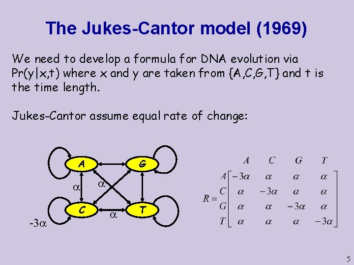
The Jukes-Cantor model (1969) We need to develop a formula for DNA evolution via Pr(y|x, t) where x and y are taken from {A, C, G, T} and t is the time length. Jukes-Cantor assume equal rate of change: A C -3 G T 5

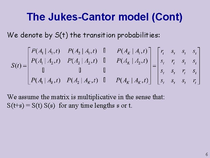
The Jukes-Cantor model (Cont) We denote by S(t) the transition probabilities: We assume the matrix is multiplicative in the sense that: S(t+s) = S(t) S(s) for any time lengths s or t. 6

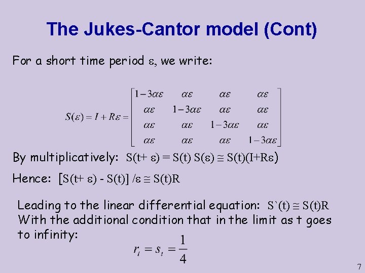
The Jukes-Cantor model (Cont) For a short time period , we write: By multiplicatively: S(t+ ) = S(t) S( ) S(t)(I+R ) Hence: [S(t+ ) - S(t)] / S(t)R Leading to the linear differential equation: S`(t) S(t)R With the additional condition that in the limit as t goes to infinity: 7

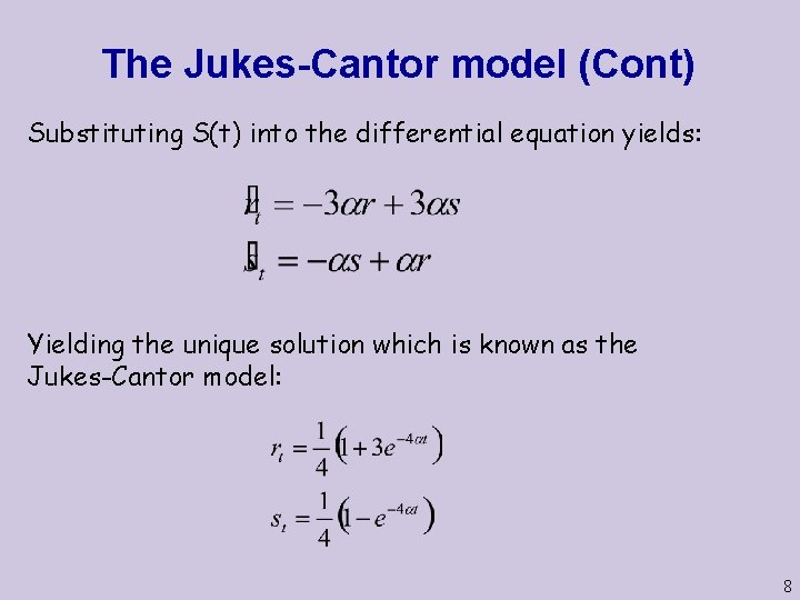
The Jukes-Cantor model (Cont) Substituting S(t) into the differential equation yields: Yielding the unique solution which is known as the Jukes-Cantor model: 8

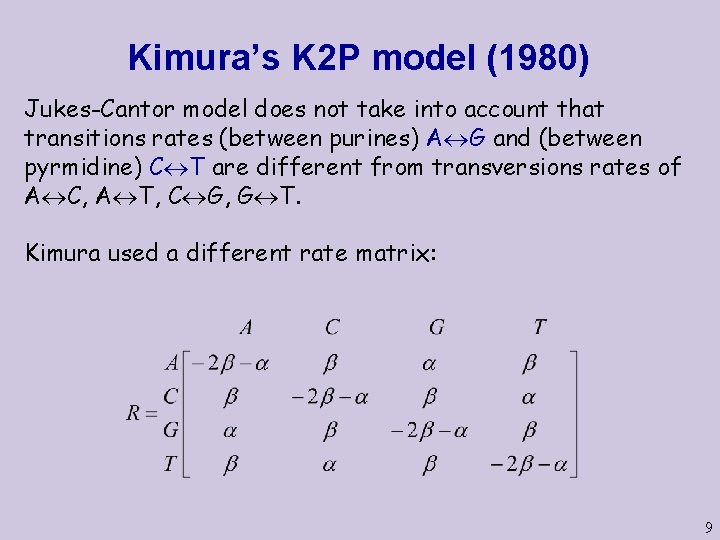
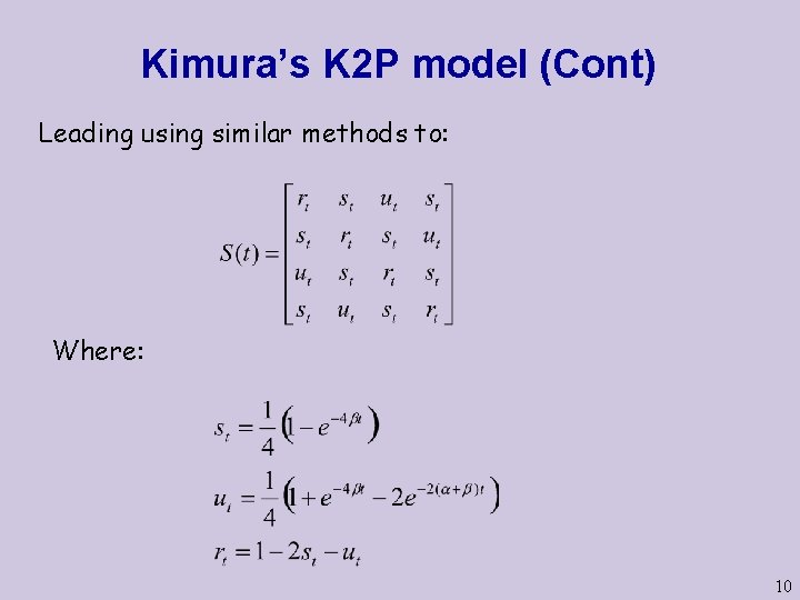
Kimura’s K 2 P model (1980) Jukes-Cantor model does not take into account that transitions rates (between purines) A G and (between pyrmidine) C T are different from transversions rates of A C, A T, C G, G T. Kimura used a different rate matrix: 9

Kimura’s K 2 P model (Cont) Leading using similar methods to: Where: 10

Hasegawa, Kishino & Yano model (1985) Still the equilibrium probabilities are all ¼ in Kimura’s model, despite the facts that in many organisms show strong bias in their AT to CG ratio. HKY’s model takes care of this. Also Felsenstein’s model F 84 takes care of this problem. There are other models as well, the most general of which is a matrix where all rates of change are distinct (12 parameters). The following chart shows relationships among most used models. 11