
Photometry Virtual Observatory Gijs Verdoes Kleijn Kapteyn Institute
Photometry & Virtual Observatory Gijs Verdoes Kleijn Kapteyn Institute, room 147 verdoes@astro. rug. nl 050 -3638326
Concepts discussed • The light path • Photometric calibration – Standard systems – Calibration procedures • Photometric calibration & VO • In other words: physics of interaction over light path; calibration: quantifying interactions; sharing your photometry
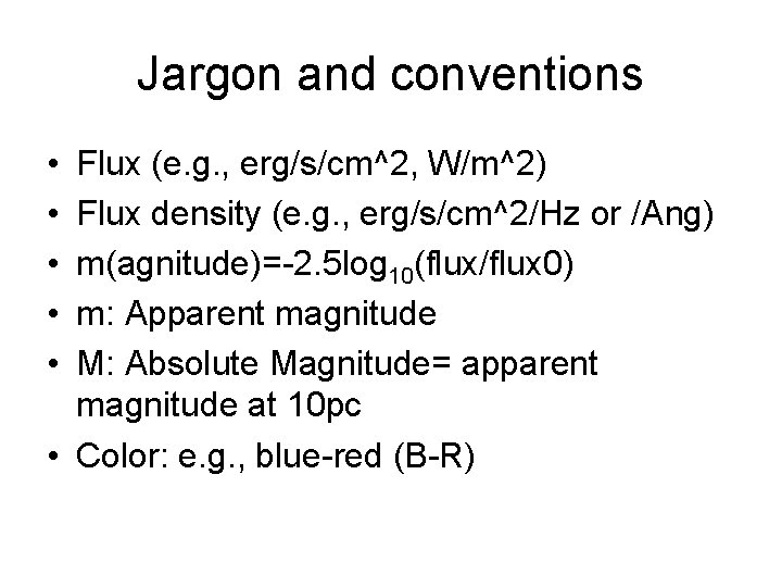
Jargon and conventions • • • Flux (e. g. , erg/s/cm^2, W/m^2) Flux density (e. g. , erg/s/cm^2/Hz or /Ang) m(agnitude)=-2. 5 log 10(flux/flux 0) m: Apparent magnitude M: Absolute Magnitude= apparent magnitude at 10 pc • Color: e. g. , blue-red (B-R)
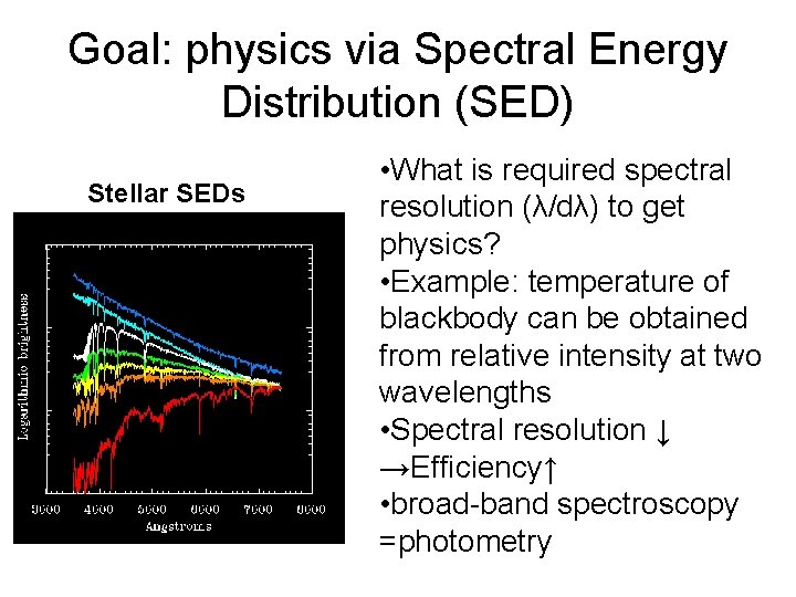
Goal: physics via Spectral Energy Distribution (SED) Stellar SEDs • What is required spectral resolution (λ/dλ) to get physics? • Example: temperature of blackbody can be obtained from relative intensity at two wavelengths • Spectral resolution ↓ →Efficiency↑ • broad-band spectroscopy =photometry
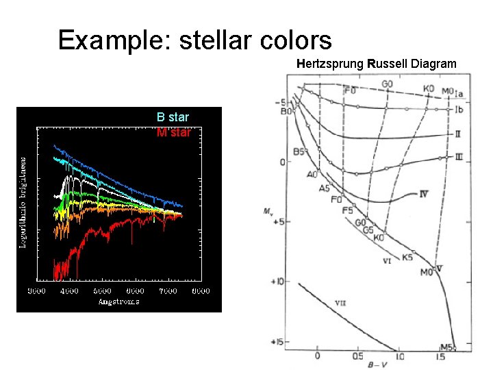
Example: stellar colors Hertzsprung Russell Diagram B star M star Hertzsprung-Russell diagram=life of star (gal=n_stars)
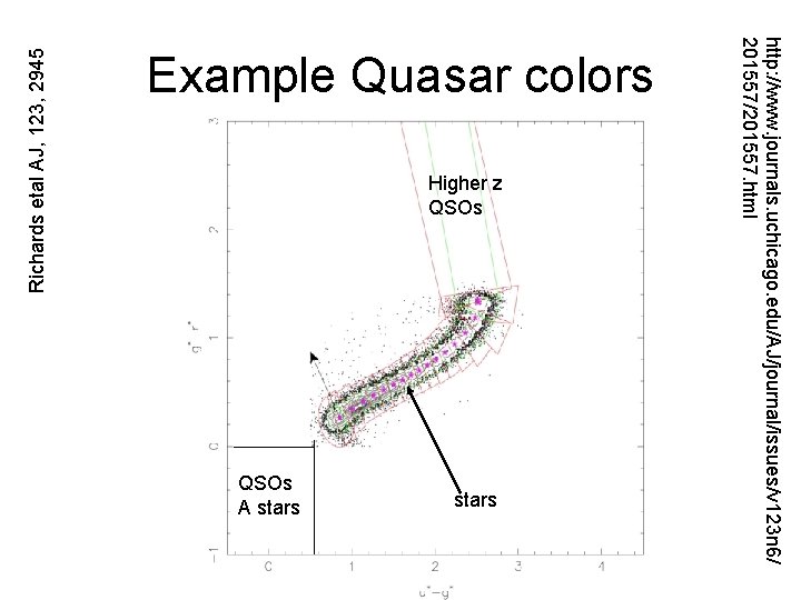
Richards etal AJ, 123, 2945 Higher z QSOs A stars http: //www. journals. uchicago. edu/AJ/journal/issues/v 123 n 6/ 201557/201557. html Example Quasar colors
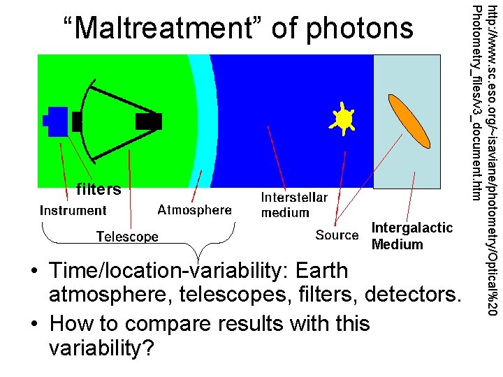
filters Intergalactic Medium • Time/location-variability: Earth atmosphere, telescopes, filters, detectors. • How to compare results with this variability? http: //www. sc. eso. org/~isaviane/photometry/Optical%20 Photometry_files/v 3_document. htm “Maltreatment” of photons
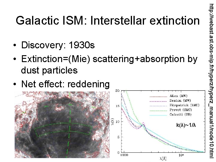
• Discovery: 1930 s • Extinction=(Mie) scattering+absorption by dust particles • Net effect: reddening k(λ)~1/λ http: //webast. obs-mip. fr/hyperz_manual 1/node 10. html Galactic ISM: Interstellar extinction
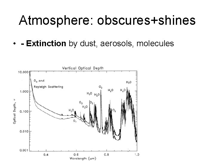
Atmosphere: obscures+shines • - Extinction by dust, aerosols, molecules
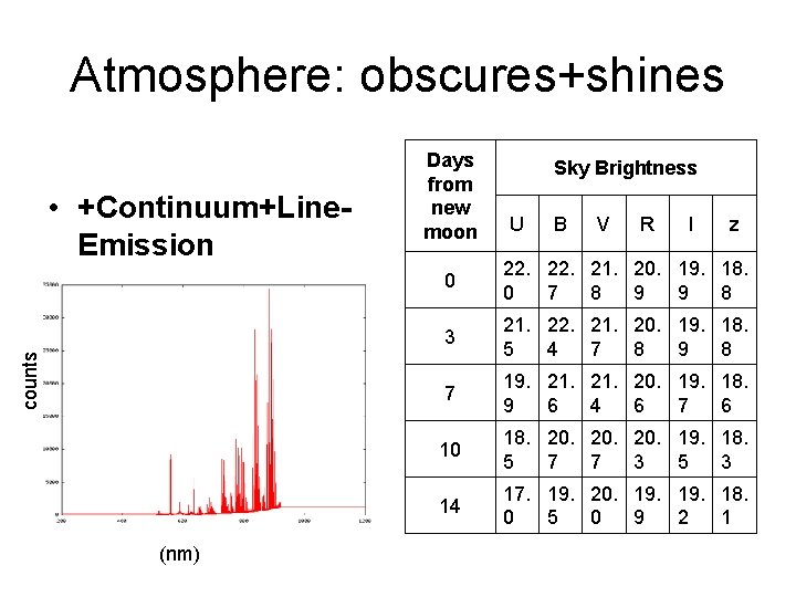
Atmosphere: obscures+shines counts • +Continuum+Line. Emission (nm) Days from new moon Sky Brightness U B V R I z 0 22. 21. 20. 19. 18. 0 7 8 9 9 8 3 21. 22. 21. 20. 19. 18. 5 4 7 8 9 8 7 19. 21. 20. 19. 18. 9 6 4 6 7 6 10 18. 20. 20. 19. 18. 5 7 7 3 5 3 14 17. 19. 20. 19. 18. 0 5 0 9 2 1
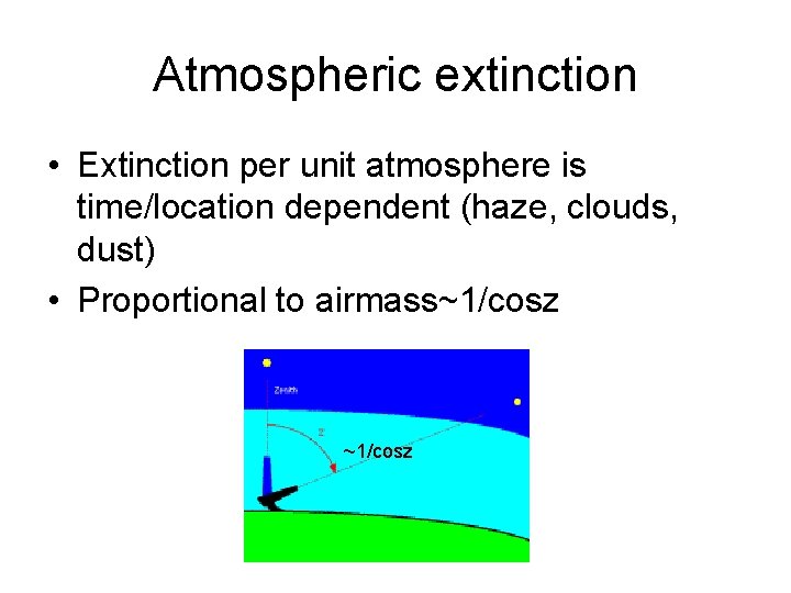
Atmospheric extinction • Extinction per unit atmosphere is time/location dependent (haze, clouds, dust) • Proportional to airmass~1/cosz
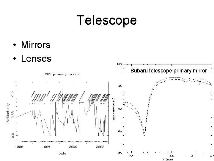
Telescope • Mirrors • Lenses Subaru telescope primary mirror
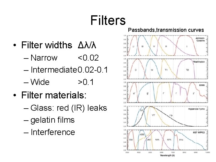
Filters • Filter widths Δλ/λ – Narrow <0. 02 – Intermediate 0. 02 -0. 1 – Wide >0. 1 • Filter materials: – Glass: red (IR) leaks – gelatin films – Interference Passbands, transmission curves
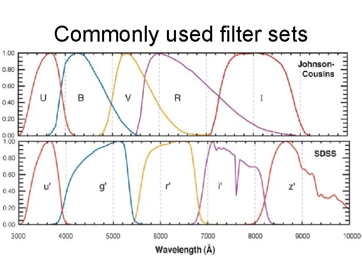
Commonly used filter sets
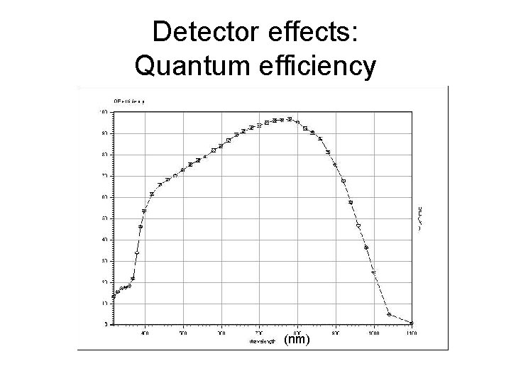
Detector effects: Quantum efficiency (nm)
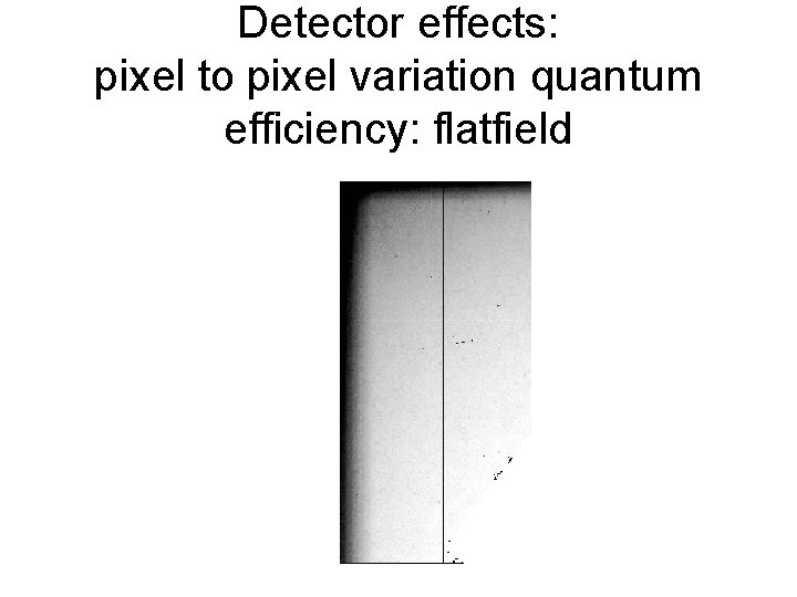
Detector effects: pixel to pixel variation quantum efficiency: flatfield
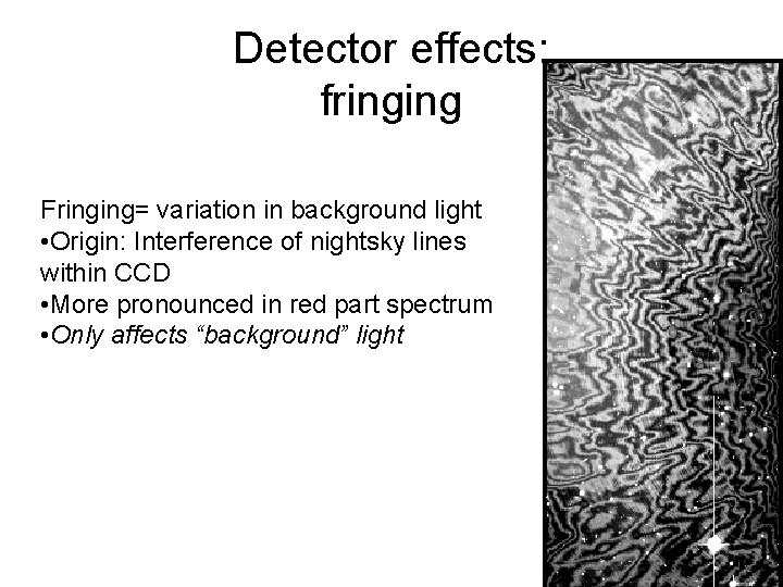
Detector effects: fringing Fringing= variation in background light • Origin: Interference of nightsky lines within CCD • More pronounced in red part spectrum • Only affects “background” light
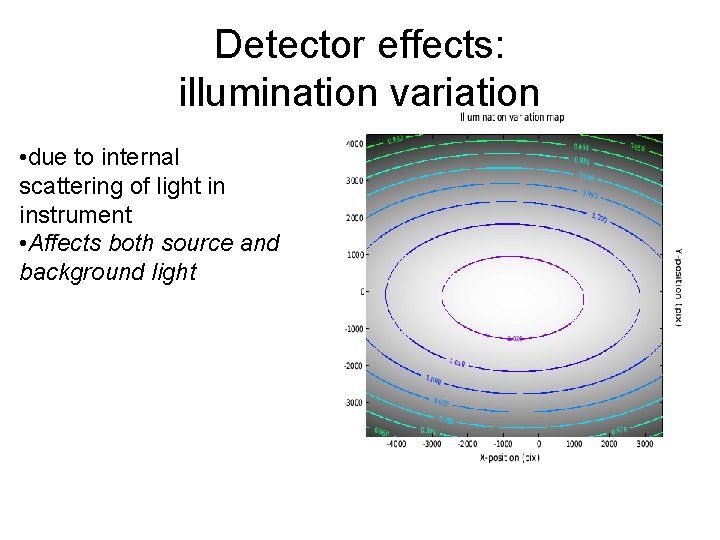
Detector effects: illumination variation • due to internal scattering of light in instrument • Affects both source and background light
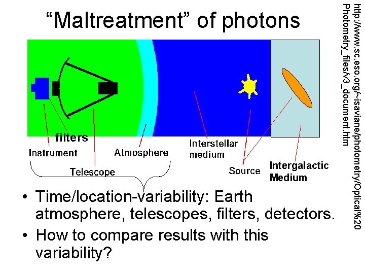
filters Intergalactic Medium • Time/location-variability: Earth atmosphere, telescopes, filters, detectors. • How to compare results with this variability? http: //www. sc. eso. org/~isaviane/photometry/Optical%20 Photometry_files/v 3_document. htm “Maltreatment” of photons
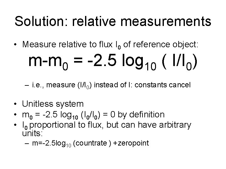
Solution: relative measurements • Measure relative to flux I 0 of reference object: m-m 0 = -2. 5 log 10 ( I/I 0) – i. e. , measure (I/I 0) instead of I: constants cancel • Unitless system • m 0 = -2. 5 log 10 (I 0/I 0) = 0 by definition • I 0 proportional to flux, but can have arbitrary units: – m=-2. 5 log 10 (countrate ) +zeropoint
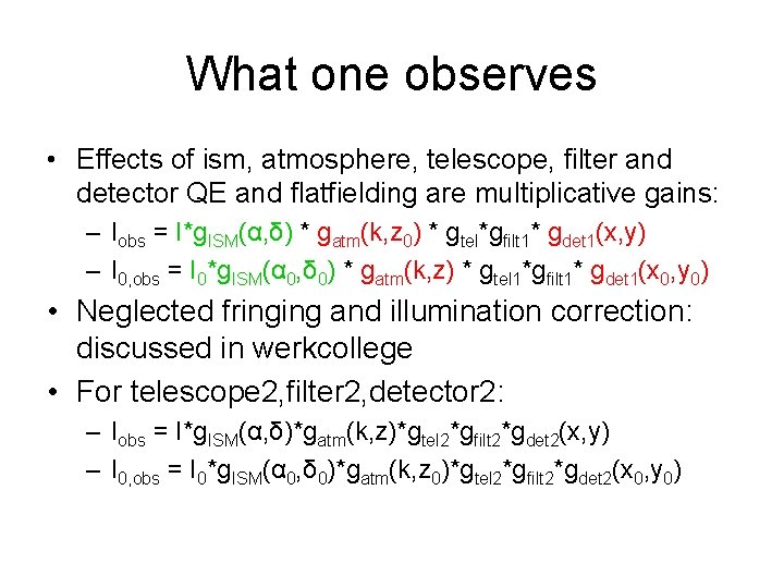
What one observes • Effects of ism, atmosphere, telescope, filter and detector QE and flatfielding are multiplicative gains: – Iobs = I*g. ISM(α, δ) * gatm(k, z 0) * gtel*gfilt 1* gdet 1(x, y) – I 0, obs = I 0*g. ISM(α 0, δ 0) * gatm(k, z) * gtel 1*gfilt 1* gdet 1(x 0, y 0) • Neglected fringing and illumination correction: discussed in werkcollege • For telescope 2, filter 2, detector 2: – Iobs = I*g. ISM(α, δ)*gatm(k, z)*gtel 2*gfilt 2*gdet 2(x, y) – I 0, obs = I 0*g. ISM(α 0, δ 0)*gatm(k, z 0)*gtel 2*gfilt 2*gdet 2(x 0, y 0)
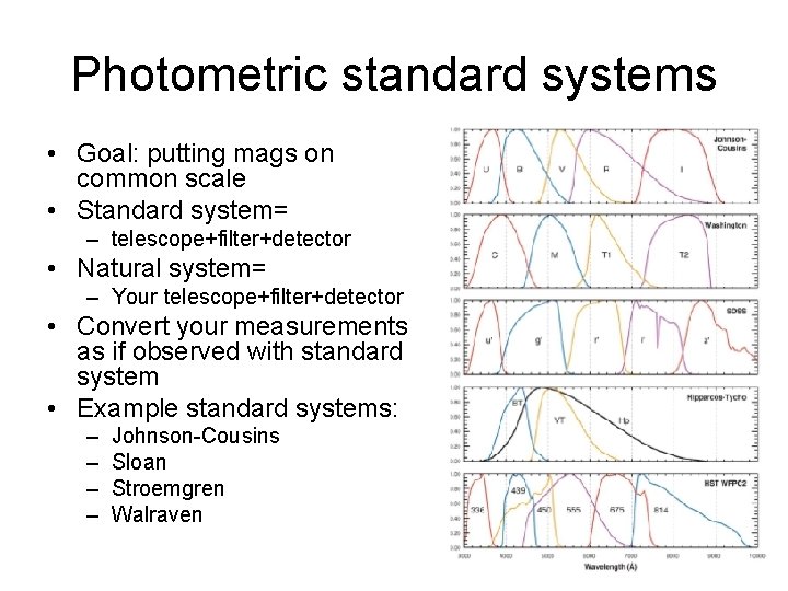
Photometric standard systems • Goal: putting mags on common scale • Standard system= – telescope+filter+detector • Natural system= – Your telescope+filter+detector • Convert your measurements as if observed with standard system • Example standard systems: – – Johnson-Cousins Sloan Stroemgren Walraven
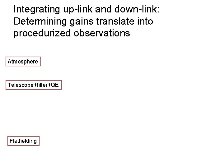
Integrating up-link and down-link: Determining gains translate into procedurized observations Atmosphere Telescope+filter+QE Flatfielding

Reflecting on design->deliver slides from previous lectures….
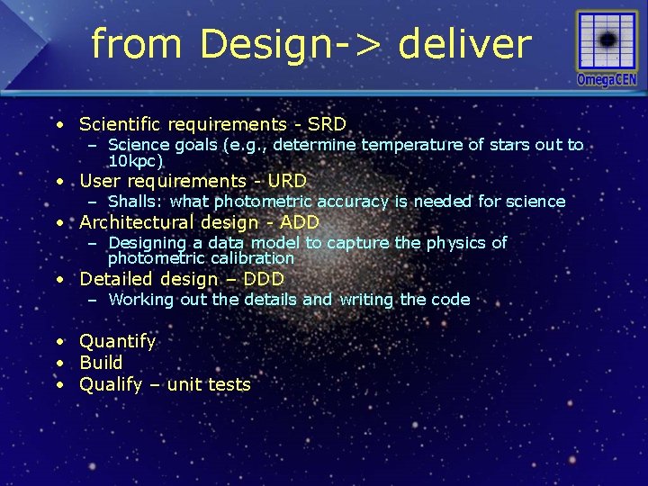
from Design-> deliver • Scientific requirements - SRD – Science goals (e. g. , determine temperature of stars out to 10 kpc) • User requirements - URD – Shalls: what photometric accuracy is needed for science • Architectural design - ADD – Designing a data model to capture the physics of photometric calibration • Detailed design – DDD – Working out the details and writing the code • Quantify • Build • Qualify – unit tests
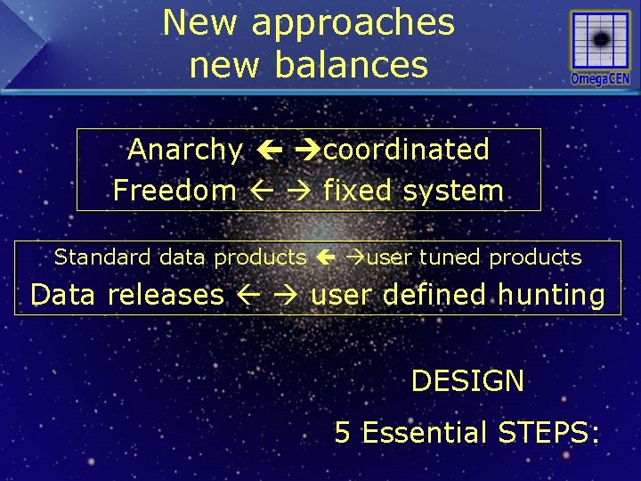
New approaches new balances Anarchy coordinated Freedom fixed system Standard data products user tuned products Data releases user defined hunting DESIGN 5 Essential STEPS:
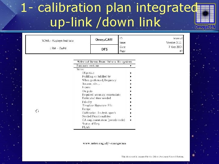
1 - calibration plan integrated up-link /down link
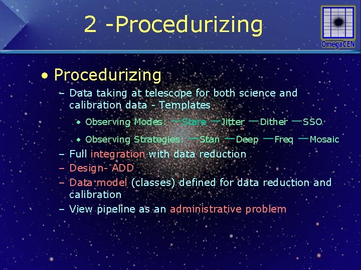
2 -Procedurizing • Procedurizing – Data taking at telescope for both science and calibration data - Templates —Stare —Jitter —Dither —SSO Observing Strategies: —Stan —Deep —Freq —Mosaic • Observing Modes: • – Full integration with data reduction – Design- ADD – Data model (classes) defined for data reduction and calibration – View pipeline as an administrative problem
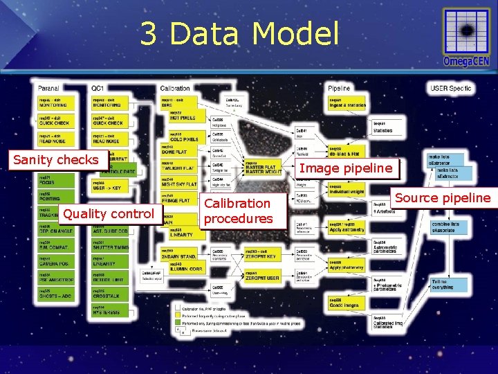
3 Data Model Sanity checks Quality control Image pipeline Calibration procedures Source pipeline
4 Integrated archive and Large Data Volume • Handling of the data is non-trivial – Pipeline data reduction – Calibration with very limited resources – Things change in time: –Physical changes (atmosphere, various gains) –Code (new methods, bugs) –Human insight in changes – Working with source lists Science can only be archive based
Photometric calibration and the VO • Now you have your result and you want to share it…. . =VO • Describing photometry universally: UCDs – Properties measurement: aperture…. . – Value and error
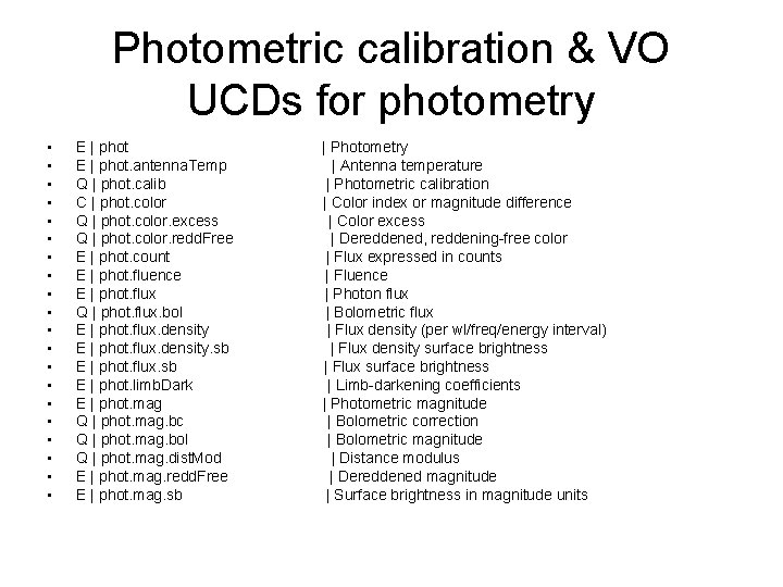
Photometric calibration & VO UCDs for photometry • • • • • E | phot | Photometry E | phot. antenna. Temp | Antenna temperature Q | phot. calib | Photometric calibration C | phot. color | Color index or magnitude difference Q | phot. color. excess | Color excess Q | phot. color. redd. Free | Dereddened, reddening-free color E | phot. count | Flux expressed in counts E | phot. fluence | Fluence E | phot. flux | Photon flux Q | phot. flux. bol | Bolometric flux E | phot. flux. density | Flux density (per wl/freq/energy interval) E | phot. flux. density. sb | Flux density surface brightness E | phot. flux. sb | Flux surface brightness E | phot. limb. Dark | Limb-darkening coefficients E | phot. mag | Photometric magnitude Q | phot. mag. bc | Bolometric correction Q | phot. mag. bol | Bolometric magnitude Q | phot. mag. dist. Mod | Distance modulus E | phot. mag. redd. Free | Dereddened magnitude E | phot. mag. sb | Surface brightness in magnitude units
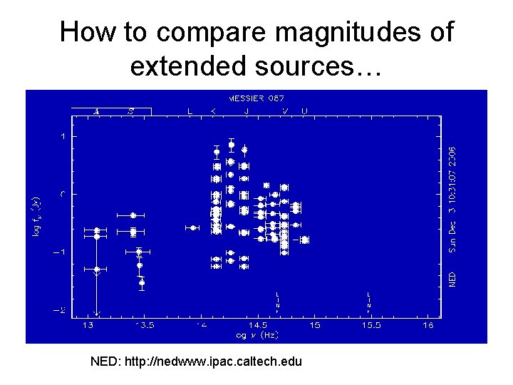
How to compare magnitudes of extended sources… NED: http: //nedwww. ipac. caltech. edu
- Slides: 34