Photo JeanFranois Dars Anne Papillault Bernoulli Random Matrix

Photo : Jean-François Dars Anne Papillault

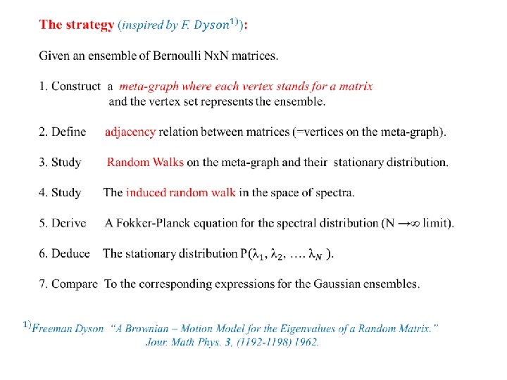
Bernoulli Random Matrix Ensembles and Random walks on Graphs With Chris Joyner In memory of Oriol, Paris March 2014 Jacob Bernoulli (1655 - 1705) Abstract The matrix elements of Bernoulli random matrices are chosen randomly from {0, 1}, subject to some symmetry requirement and in some cases subject to global constraints. The extension to the Bernoulli case, of Dyson's Brownian motion model of Gaussian ensembles, will be discussed. This will be done by considering random walks on graphs which represent these ensembles.

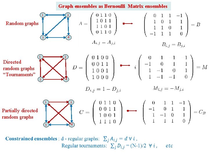
Graph ensembles as Bernoulli Matrix ensembles 1 2 3 4 Random graphs 1 2 3 4 Directed random graphs “Tournaments” 1 2 3 4 Partially directed random graphs

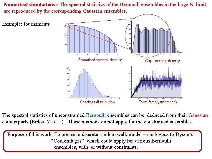
Numerical simulations : The spectral statistics of the Bernoulli ensembles in the large N limit are reproduced by the corresponding Gaussian ensembles. Example: tournaments Smoothed spectral density Spacings distribution Gap spectral density Form factor(smoothed) The spectral statistics of unconstrained Bernoulli ensembles can be deduced from their Gaussian counterparts (Erdos, Yao, …). These methods do not apply for the constrained ensembles. Purpose of this work: To present a discrete random walk model – analogous to Dyson’s “Coulomb gas” which could apply for various Bernoulli ensembles, with or without constraints.

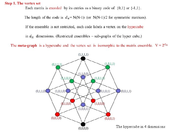
(1, 1, 1, 1) (1, 0, 1, 1) (0, 1, 1, 1) (1, 1, 0, 0) (1, 1, 0, 1) (0, 1, 1, 0) (1, 0, 1, 1) (1, 0, 1, 0) (0, 1, 0, 1) (0, 1, 0, 0) (0, 0, 1, 1) (1, 0, 0, 0) (1, 0, 0, 1) (0, 0, 1, 0) (0, 0, 0, 1) (0, 0, 0, 0) The hypercube in 4 dimensions

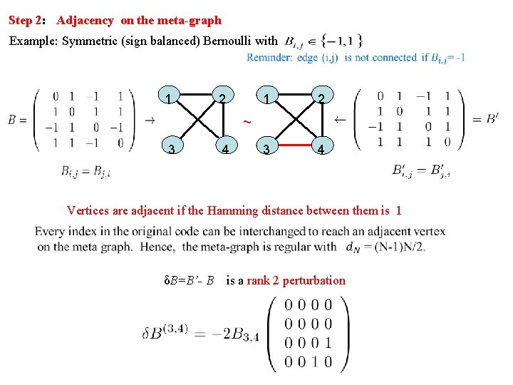
Step 2: Adjacency on the meta-graph Example: Symmetric (sign balanced) Bernoulli with 1 2 3 4 ~ 3 4 Vertices are adjacent if the Hamming distance between them is 1 δB=B’- B is a rank 2 perturbation

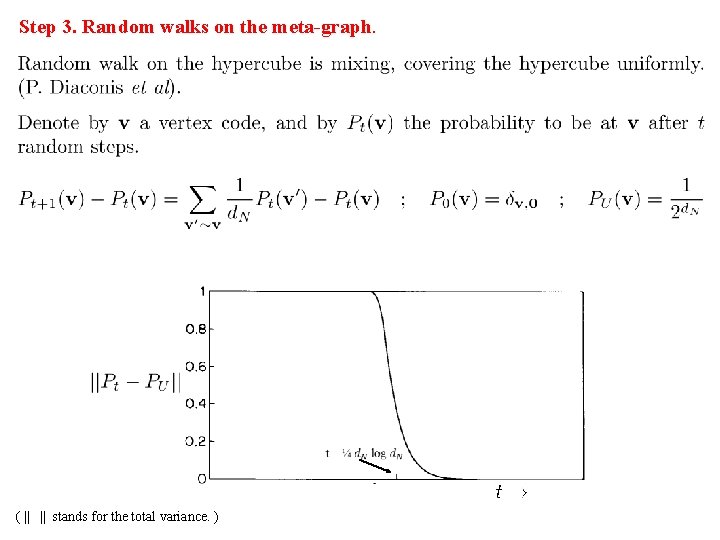
Step 3. Random walks on the meta-graph. ( || || stands for the total variance. )

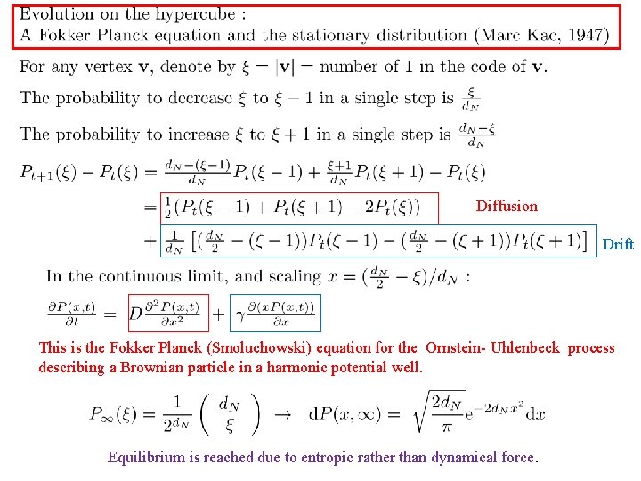
Diffusion Drift This is the Fokker Planck (Smoluchowski) equation for the Ornstein- Uhlenbeck process describing a Brownian particle in a harmonic potential well. Equilibrium is reached due to entropic rather than dynamical force.

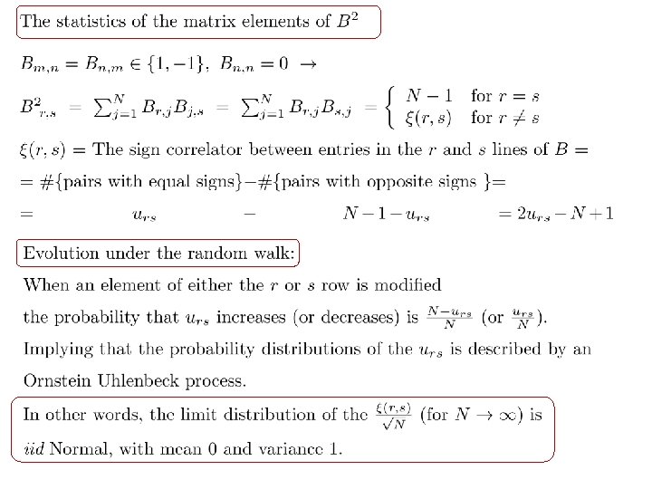
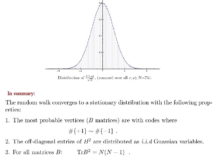
In summary:

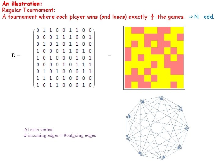
An illustration: Regular Tournament: A tournament where each player wins (and loses) exactly ½ the games. -> N odd. D= = At each vertex: # incoming edges = #outgoing edges

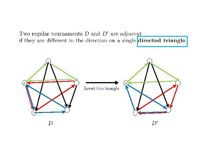
Invert blue triangle

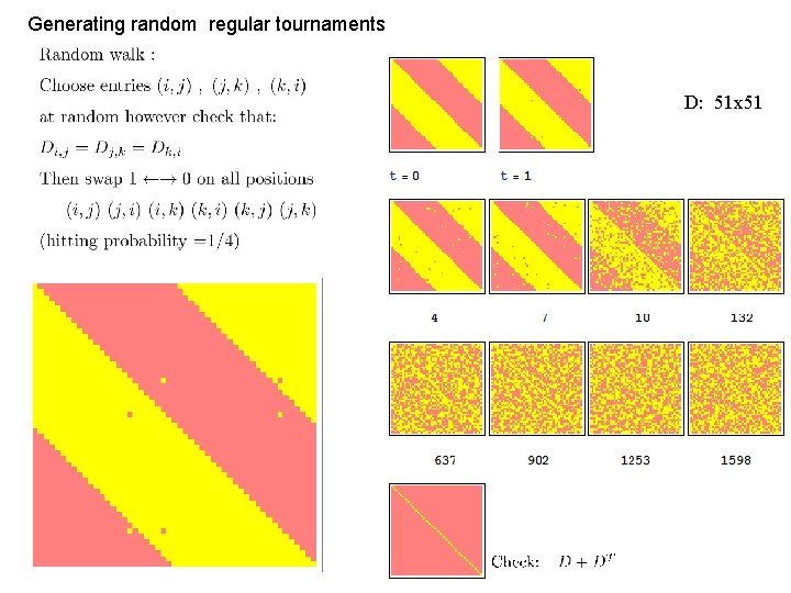
Generating random regular tournaments D: 51 x 51

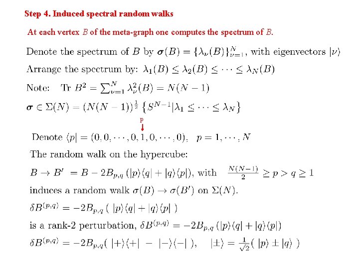
Step 4. Induced spectral random walks At each vertex B of the meta-graph one computes the spectrum of B. p

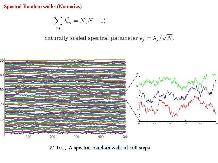
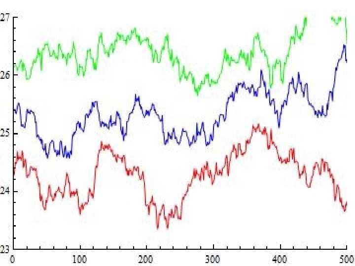
Spectral Random walks (Numerics) N=101, A spectral random walk of 500 steps

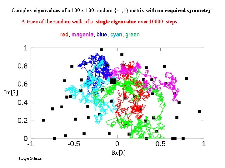
Complex eigenvalues of a 100 x 100 random {-1, 1} matrix with no required symmetry A trace of the random walk of a single eigenvalue over 10000 steps. red, magenta, blue, cyan, green Im[λ] Re[λ] Holger Schanz.

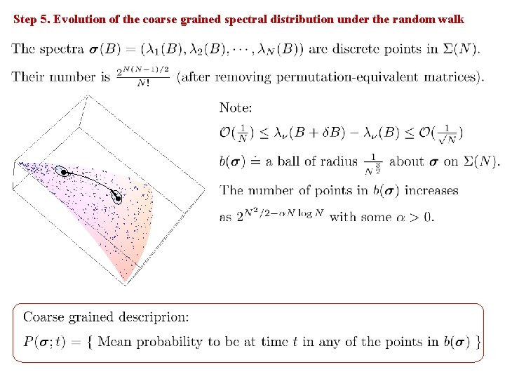
Step 5. Evolution of the coarse grained spectral distribution under the random walk

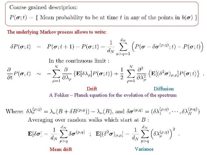
The underlying Markov process allows to write: Drift Diffusion A Fokker – Planck equation for the evolution of the spectrum Mean drift Variance

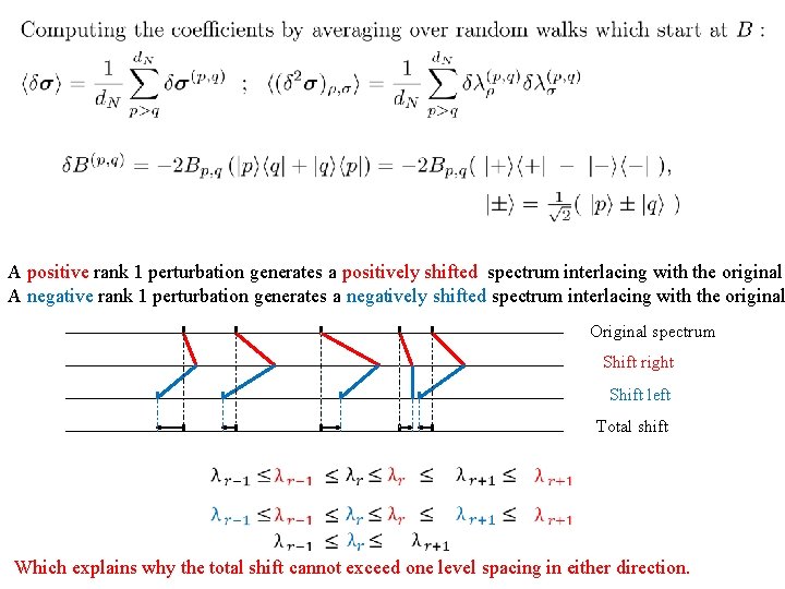
A positive rank 1 perturbation generates a positively shifted spectrum interlacing with the original A negative rank 1 perturbation generates a negatively shifted spectrum interlacing with the original Original spectrum Shift right Shift left Total shift Which explains why the total shift cannot exceed one level spacing in either direction.

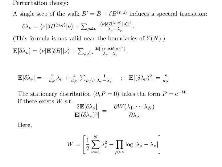
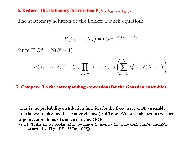
7. Compare To the corresponding expressions for the Gaussian ensembles. This is the probability distribution function for the fixed trace GOE ensemble. It is known to display the semi-circle law (and Tracy Widom statistics) as well as k point correlations of the unrestricted GOE. (e. g, F. Goetze and M. Gordin: Limit correlation functions for fixed trace random matrix ensembles. Comm. Math. Phys. 215, 683 -706 (2008))

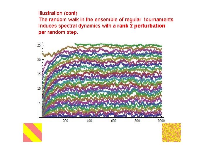
Illustration (cont) The random walk in the ensemble of regular tournaments Induces spectral dynamics with a rank 2 perturbation per random step.

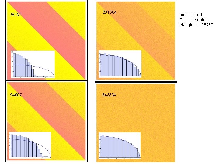
28257 94007 281584 843334 nmax = 1501 # of attempted triangles 1125750

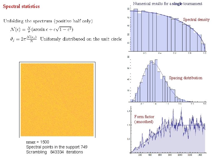
Spectral statistics Numerical results for a single tournament Spectral density Spacing distribution Form factor (smoothed) nmax = 1500 Spectral points in the support 749 Scrambling 843334 iterations

Summary: 1 The derivation above is not entirely rigorous. 2. The same method applies with some minor modifications for the unrestricted ensembles (Tournaments, {0, 1} matrices). 3. The eigenvectors distributions are not derived or assumed. 4. Work on the restricted ensembles (d-regular, regular tournaments) is in progress. (With Chris Joyner) Thank you for your attention