PHIL 201 Chapter 13 Statistical Arguments Evaluating Statistical

PHIL 201 Chapter 13 Statistical Arguments

Evaluating Statistical Arguments • We are frequently offered arguments employing statistical claims as premises. • To evaluate such arguments, we must be able to interpret the statistics on which they are based and evaluate the support that they provide for the conclusion. • There a number of challenges to such interpretation and evaluation. • Statements expressing averages and percentages are often ambiguous. • This ambiguity allows for deception (deliberate or accidental).

Inductive Generalizations • Inductive Generalization: argument that an entire class of things has the characteristics of a subset of the class. • All IGs have some basic features in common: • A conclusion describing what is inferred about all or many members of a larger group, called the population. • A premise or premises describing a subset of the population, called the sample. • The characteristic of the sample held to be true of the entire population. • The basic form of the IG is: All observed A’s are f. Thus, probably all A’s are f.

Statistical Generalizations • A specialized form of the IG is called a Statistical Generalization: X percent of observed A’s are f. Therefore, probably X percent of all A’s are f. • How does the notion of Inductive strength function in terms of inductive generalizations? In general, the more representative the sample, the stronger the generalization. • What makes a sample representative? A sample is representative of a population to the degree that the target characteristics found in the sample occur with the same frequency/proportion as they occur in the population. • In order to determine if a sample is representative we need to know 1)the characteristics that occur in the population; 2)whether those characteristics are relevant to the target characteristic.

Representativeness and Bias • Confidence in statistical generalizations is a function of the representativeness of the sample from which they are drawn. • Samples that are not representative are said to be biased samples. • Determiners: • • • Whether the sample is randomly selected The size of the sample Psychological factors • If you are presented with a statistical generalization relying on data generated by studies that may be biased samples, your confidence in the conclusion should be weak. • Ask yourself: Do you know if the sample is random? Is the sample size appropriate? What if any psychological factors may be in play?

Randomness and Sample Size • Random samples are when every member of the population has an equal chance of being selected. • Literary Digest 1936 Presidential Election Poll predicted that Alf Landon would beat Franklin Roosevelt. The sample was collected from subscribers, supplemented by automobile registration records and telephone users. Why wasn’t this random? • A second concern is sample size. Assuming a random sample, the larger the sample the more representative it is likely to be. • The representativeness of sampling size is expressed through the concept of sampling error: the difference between the relative frequency with which some characteristic occurs in a sample and the relative frequency this characteristic appears in the population. Adequate sample size is a function of the size of the population and the specification of the tolerable sampling error. • • • The relationship between sample size and population size is not linear. Though most reliable polling presupposes a sampling error (as expressed by margin of error) of 5% or less, unless the poll you are considering specifies it’s sampling error, it should be ignored.

Psychological Factors • Psychological factors can play a role in sample representativeness when the population under consideration consists of human beings. • Humans are notorious for responding to polling/surveys with a range of predictable biases. • The content and form of questions often alters the results of data collection. • It’s important to recognize that its not only the psychological biases of the respondents, but also of the surveyors that can affect the outcome of the survey. • Imagine a study comparing the effectiveness of surgical procedures. The patients can be kept in ignorance, but the surgeons cannot. • One approach to dealing with psychological factors is the “double blind” study: questions designed in such a way that neither the respondent nor the surveyor can identify the ‘right’ way to answer the question.

Exercise 13 A Why Women Choose Manly Men By FREAKONOMICS, 4/7/10 Researchers at the University of Aberdeen’s Face Research Laboratory have some news of interest for particularly “masculine”-looking men. Almost 4, 800 women from around the world logged on to the organization’s online lab over the past year, viewed 20 pairs of male faces (similar, but one slightly more masculine than the other), and expressed their preferences. The Wall Street Journal reports on what the researchers found: “They could predict how masculine a woman likes her men based on her nation’s World Health Organization statistics for mortality rates, life expectancy and the impact of communicable disease. ” In short, women in less healthy countries preferred more masculine men, perhaps for their evolutionary advantages (testosterone is linked to health). So if you’re blessed or burdened with a short, broad face and a strong jawline, you might want to think about moving to Argentina.

Exercise 13 A • Answer Sample: 4, 800 women from around the world. Population: All women. Sample size: This is a very large sample, but we need to know more about how the women were selected. Potential bias: The sample excludes women who do not have access to the Internet and this organization’s online lab. Also, only 20 pairs of male faces were viewed and compared, allowing for the possibility that including additional male faces, fitting alternative definitions of “masculine, ” might have led to different results. Randomness: This is not a random sample, because not every woman had an equal chance of getting into the sample. This reduces the likelihood that the sample is representative of the population.

The Meaning of “Average” • The term ‘average’ had three distinct mathematical senses. Unless you know which particular sense is being invoked at any time, you should hesitate before drawing any conclusions about an ‘average. ’ • MEAN • The arithmetical average • Divide the sum of the individual values by the number of values in the set • MEDIAN • The middle point when the data are arranged in ascending order • The point at which there is an equal number of data above and below. • MODE • The value that occurs with greatest frequency

Exercise 13 B Example (13 B I #2) [3, 5, 7, 9, 11, 11] Answer Mean: 8. 14 Median: 9 Mode: 11

Dispersion • Knowing the average (in any one of the three senses) of a set of data can be useful. But, often the average alone is insufficient basis to draw conclusions about the significance of the set. • The import of the average can differ depending on how the data are distributed around the average. • To get a better sense of the significance of a claim about averages, we employ the concept of Dispersion: how spread out or diverse the data are in regard to numerical value.

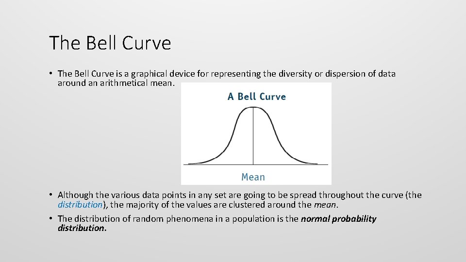
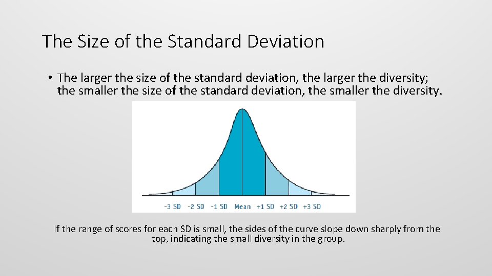
The Bell Curve • The Bell Curve is a graphical device for representing the diversity or dispersion of data around an arithmetical mean. • Although the various data points in any set are going to be spread throughout the curve (the distribution), the majority of the values are clustered around the mean. • The distribution of random phenomena in a population is the normal probability distribution.

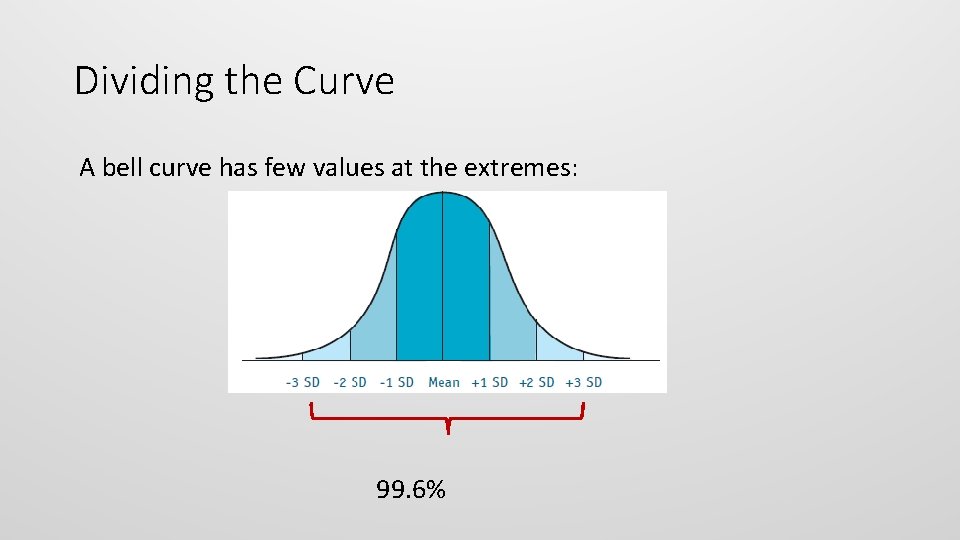
Dividing the Curve A bell curve has few values at the extremes: 99. 6%

The Size of the Standard Deviation • The larger the size of the standard deviation, the larger the diversity; the smaller the size of the standard deviation, the smaller the diversity. If the range of scores for each SD is small, the sides of the curve slope down sharply from the top, indicating the small diversity in the group.

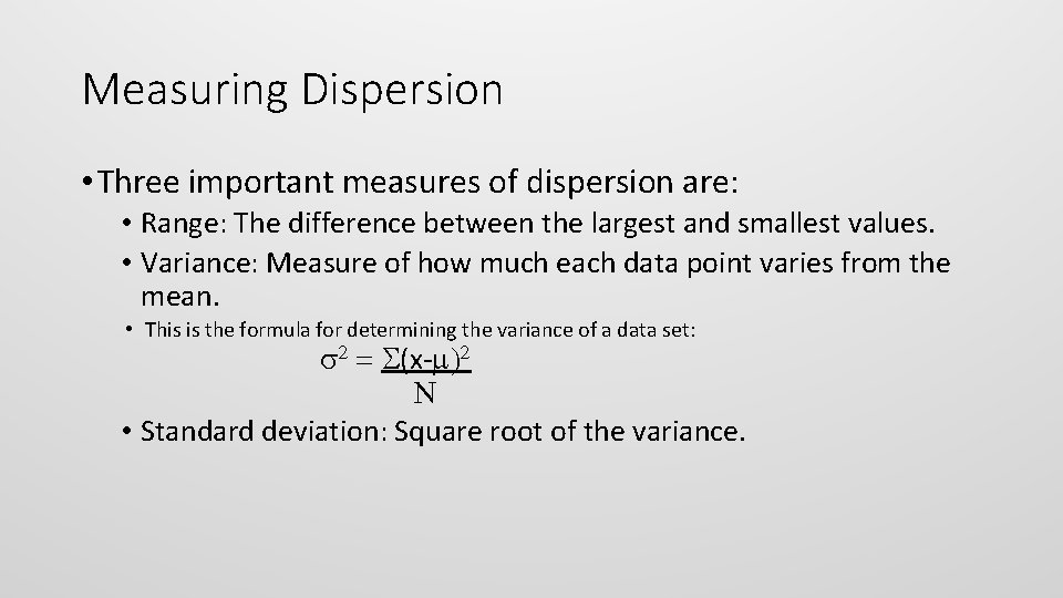
Measuring Dispersion • Three important measures of dispersion are: • Range: The difference between the largest and smallest values. • Variance: Measure of how much each data point varies from the mean. • This is the formula for determining the variance of a data set: s 2 = S(x-m)2 N • Standard deviation: Square root of the variance.

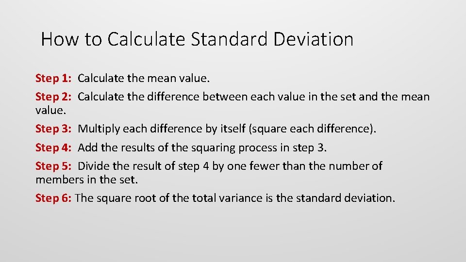
How to Calculate Standard Deviation Step 1: Calculate the mean value. Step 2: Calculate the difference between each value in the set and the mean value. Step 3: Multiply each difference by itself (square each difference). Step 4: Add the results of the squaring process in step 3. Step 5: Divide the result of step 4 by one fewer than the number of members in the set. Step 6: The square root of the total variance is the standard deviation.

Exercise 13 C Example (13 C I #2) [3, 5, 7, 9, 11, 11] Answer The standard deviation is 3. 24. Step 1: Step 2: Step 3: Step 4: Step 5: Step 6: 8. 14 -5. 14; -3. 14; -1. 14; 0. 86; 2. 86 26. 42; 9. 86; 1. 3; 0. 74; 8. 18; 8. 18 62. 86 10. 48 3. 24

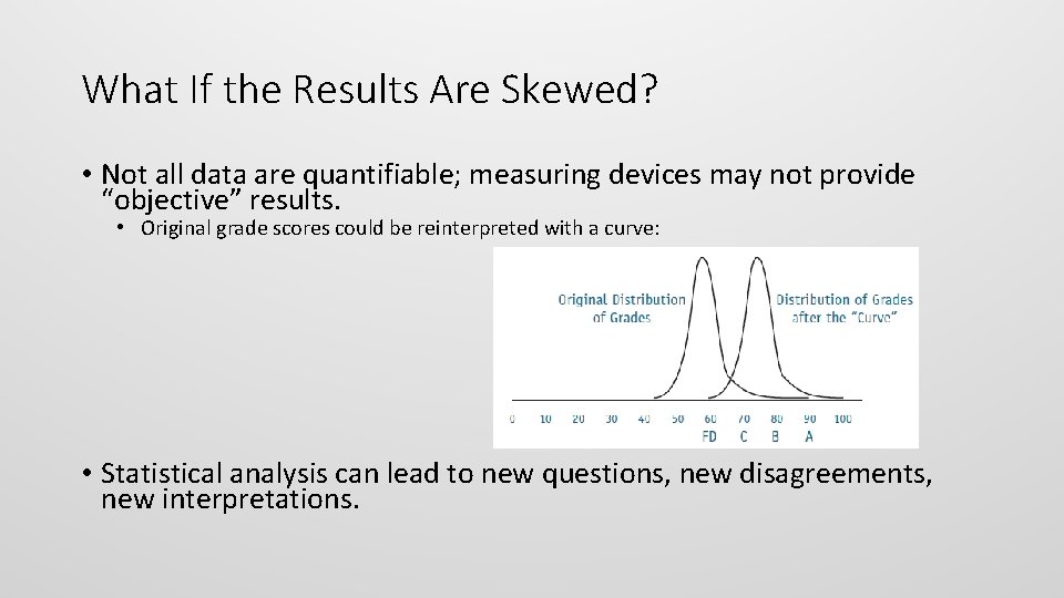
What If the Results Are Skewed? • Not all data are quantifiable; measuring devices may not provide “objective” results. • Original grade scores could be reinterpreted with a curve: • Statistical analysis can lead to new questions, new disagreements, new interpretations.

The Misuse of Statistics • Statistics can mislead either intentionally or unintentionally. • As has already been noted, unless you have the relevant information necessary to interpret statistical claims (representativeness, variance/standard deviation of the data set), those claims provide very weak support for any conclusion. • You also need to be wary of mistaking quantitative terms and qualitative terms. • Kanye is one of the best selling hip hop artists. • This is a quantitative claim and should be evaluated using appropriate standardized measures. • Kanye is a musical genius. • This is a quantitative claim, and cannot be evaluated merely on the basis of album sales, etc. . • Kanye has lost his damn mind. • This is a qualitative claim and also cannot be evaluated using appropriate standardized measures, though his twitter feed provides one source of insight.

Exercise 13 E #2 A study finds that Best Actress Oscar winners have a 63% chance of their marriages ending sooner than nonwinners. The median marriage duration was 4. 3 years; 9. 5 for nonwinners. Analysis: The group of Best Actress Oscar winners is quite small, and the group of nonwinners is at least four times as large. In addition, the two groups probably differ in many ways other than being Oscar winners. Also, we are not told the mean value and the standard deviation; therefore, without that information, we cannot determine the amount of diversity in the sets. As a result, any conclusion drawn from the data is going to be only very weakly supported by the statistical claims made in the argument, and any such argument would be weak.