Phase Transitions of a Super Quantum Mechanical Matrix

"Phase Transitions of a (Super) Quantum Mechanical Matrix Model with a Chemical Potential in terms of partial deconfinement" (ar. Xiv: 1707. 02898) Takehiro Azuma (Setsunan Univ. ) TIFR seminar 2020/1/2, 14: 30 -15: 30 with Pallab Basu (Wits) and Prasant Samantray (IUCAA)

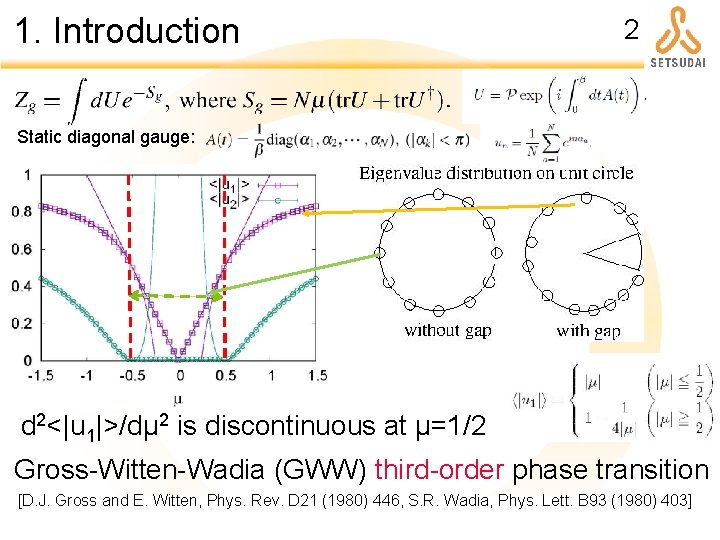
1. Introduction 2 Static diagonal gauge: d 2<|u 1|>/dμ 2 is discontinuous at μ=1/2 Gross-Witten-Wadia (GWW) third-order phase transition [D. J. Gross and E. Witten, Phys. Rev. D 21 (1980) 446, S. R. Wadia, Phys. Lett. B 93 (1980) 403]

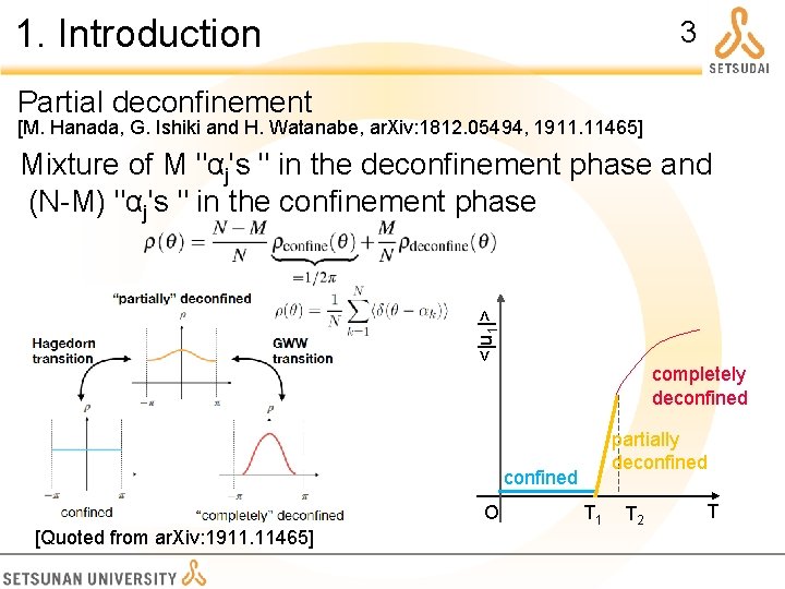
1. Introduction 3 Partial deconfinement [M. Hanada, G. Ishiki and H. Watanabe, ar. Xiv: 1812. 05494, 1911. 11465] <|u 1|> Mixture of M "αj's " in the deconfinement phase and (N-M) "αj's " in the confinement phase completely deconfined partially deconfined O [Quoted from ar. Xiv: 1911. 11465] T 1 T 2 T

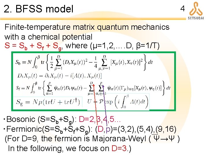
2. BFSS model 4 Finite-temperature matrix quantum mechanics with a chemical potential S = Sb + Sf + Sg, where (μ=1, 2, …. D, β=1/T) ・Bosonic (S=Sb+Sg): D=2, 3, 4, 5… ・Fermionic(S=Sb+Sf+Sg): (D, p)=(3, 2), (5, 4), (9, 16) (For D=9, the fermion is Majorana-Weyl ( Ψ→Ψ ) 　In the following, we focus on D=3. )

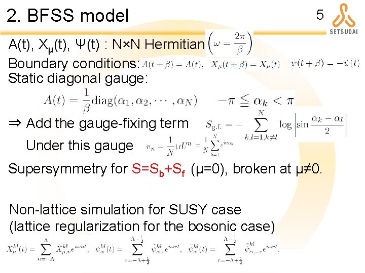
2. BFSS model 5 A(t), Xμ(t), Ψ(t) : N×N Hermitian matrix Boundary conditions: Static diagonal gauge: ⇒ Add the gauge-fixing term Under this gauge Supersymmetry for S=Sb+Sf　(μ=0), broken at μ≠ 0. Non-lattice simulation for SUSY case (lattice regularization for the bosonic case)

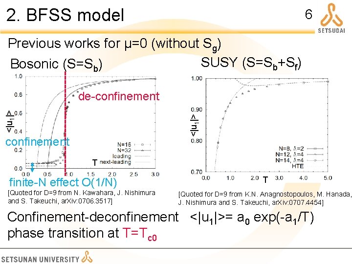
2. BFSS model 6 Previous works for μ=0 (without Sg) SUSY (S=Sb+Sf) Bosonic (S=Sb) <|u 1|> de-confinement T finite-N effect O(1/N) [Quoted for D=9 from N. Kawahara, J. Nishimura and S. Takeuchi, ar. Xiv: 0706. 3517] T [Quoted for D=9 from K. N. Anagnostopoulos, M. Hanada, J. Nishimura and S. Takeuchi, ar. Xiv: 0707. 4454] Confinement-deconfinement <|u 1|>= a 0 exp(-a 1/T) phase transition at T=Tc 0

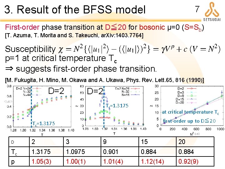
3. Result of the BFSS model 7 First-order phase transition at D≦ 20 for bosonic μ=0 (S=Sb) [T. Azuma, T. Morita and S. Takeuchi, ar. Xiv: 1403. 7764] Susceptibility p=1 at critical temperature Tc ⇒ suggests first-order phase transition. [M. Fukugita, H. Mino, M. Okawa and A. Ukawa, Phys. Rev. Lett. 65, 816 (1990)] D=2 Tc=1. 3175 at critical temperature Tc first-order up to D≦ 20 Tc=1. 3175 D 2 3 9 15 20 Tc 1. 3175 1. 0975 0. 901 0. 884 p 1. 05(3) 1. 00(1) 1. 01(4) 1. 12(14) 0. 92(9)

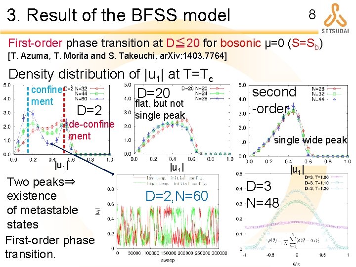
3. Result of the BFSS model 8 First-order phase transition at D≦ 20 for bosonic μ=0 (S=Sb) [T. Azuma, T. Morita and S. Takeuchi, ar. Xiv: 1403. 7764] Density distribution of |u 1| at T=Tc confine D=20 ment flat, but not D=2 single peak de-confine ment |u 1| Two peaks⇒ existence of metastable states First-order phase transition. second -order single wide peak |u 1| D=2, N=60 |u 1| D=3 N=48

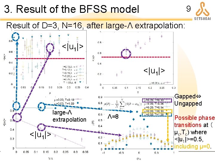
3. Result of the BFSS model 9 Result of D=3, N=16, after large-Λ extrapolation: <|u 1|> Gapped⇔ Ungapped large-Λ extrapolation <|u 1|> Λ=8 Possible phase transitions at （ μc, Tc) where <|u 1|>=0. 5, including μ=0.

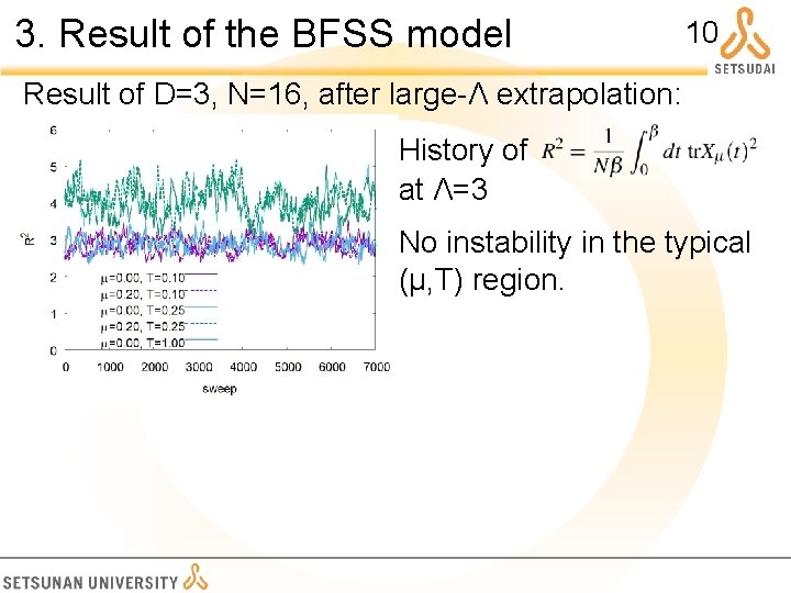
3. Result of the BFSS model 10 Result of D=3, N=16, after large-Λ extrapolation: History of at Λ=3 No instability in the typical (μ, T) region.

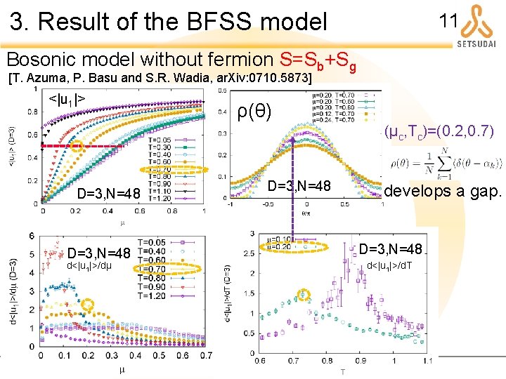
3. Result of the BFSS model 11 Bosonic model without fermion S=Sb+Sg [T. Azuma, P. Basu and S. R. Wadia, ar. Xiv: 0710. 5873] <|u 1|> ρ(θ) (μc, Tc)=(0. 2, 0. 7) D=3, N=48 d<|u 1|>/dμ D=3, N=48 develops a gap. D=3, N=48 d<|u 1|>/d. T

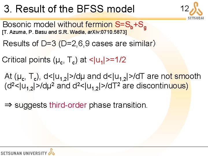
3. Result of the BFSS model 12 Bosonic model without fermion S=Sb+Sg [T. Azuma, P. Basu and S. R. Wadia, ar. Xiv: 0710. 5873] Results of D=3 (D=2, 6, 9 cases are similar） Critical points (μc, Tc) at <|u 1|>=1/2 At (μc, Tc), d<|u 1, 2|>/dμ and d<|u 1, 2|>/d. T are not smooth (d 2<|u 1, 2|>/dμ 2 and d 2<|u 1, 2|>/d. T 2 are discontinuous) ⇒ suggests third-order phase transition.

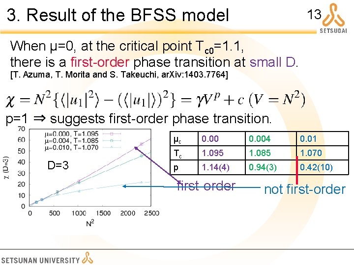
3. Result of the BFSS model 13 When μ=0, at the critical point Tc 0=1. 1, there is a first-order phase transition at small D. [T. Azuma, T. Morita and S. Takeuchi, ar. Xiv: 1403. 7764] p=1 ⇒ suggests first-order phase transition. D=3 μc 0. 004 0. 01 Tc 1. 095 1. 085 1. 070 p 1. 14(4) 0. 94(3) 0. 42(10) first-order not first-order

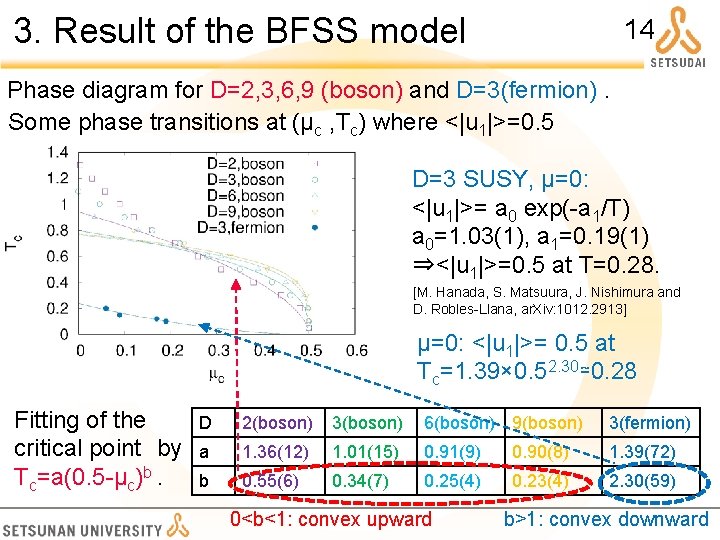
3. Result of the BFSS model 14 Phase diagram for D=2, 3, 6, 9 (boson) and D=3(fermion). Some phase transitions at (μc , Tc) where <|u 1|>=0. 5 D=3 SUSY, μ=0: <|u 1|>= a 0 exp(-a 1/T) a 0=1. 03(1), a 1=0. 19(1) ⇒<|u 1|>=0. 5 at T=0. 28. [M. Hanada, S. Matsuura, J. Nishimura and D. Robles-Llana, ar. Xiv: 1012. 2913] μ=0: <|u 1|>= 0. 5 at Tc=1. 39× 0. 52. 30≃0. 28 Fitting of the critical point　by Tc=a(0. 5 -μc)b. D 2(boson) 3(boson) 6(boson) 9(boson) 3(fermion) a 1. 36(12) 1. 01(15) 0. 91(9) 0. 90(8) 1. 39(72) b 0. 55(6) 0. 34(7) 0. 25(4) 0. 23(4) 2. 30(59) 0<b<1: convex upward b>1: convex downward

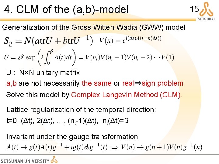
4. CLM of the (a, b)-model Generalization of the Gross-Witten-Wadia (GWW) model U : N×N unitary matrix a, b are not necessarily the same or real⇒sign problem Solve this model by Complex Langevin Method (CLM). Lattice regularization of the temporal direction: t=0, (Δt), 2(Δt), …, (nt-1)(Δt), nt(Δt)=β Invariant under the gauge transformation ⇒ 15

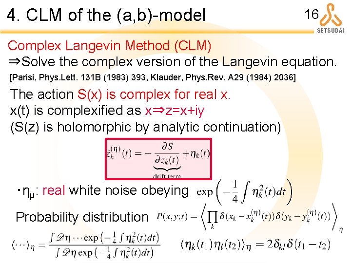
4. CLM of the (a, b)-model 16 Complex Langevin Method (CLM) ⇒Solve the complex version of the Langevin equation. [Parisi, Phys. Lett. 131 B (1983) 393, Klauder, Phys. Rev. A 29 (1984) 2036] The action S(x) is complex for real x. x(t) is complexified as x⇒z=x+iy (S(z) is holomorphic by analytic continuation) ・ημ: real white noise obeying Probability distribution

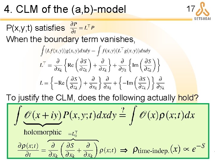
4. CLM of the (a, b)-model 17 P(x, y; t) satisfies When the boundary term vanishes, To justify the CLM, does the following actually hold? ⇒

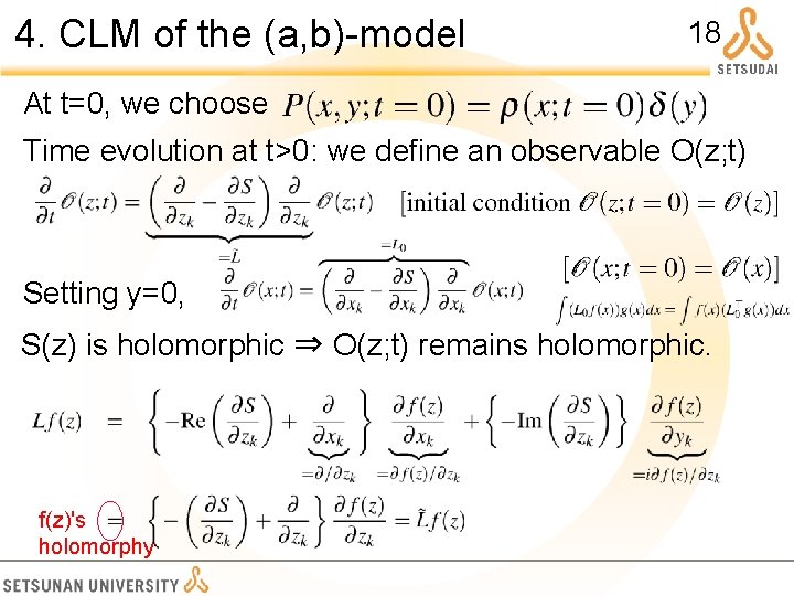
4. CLM of the (a, b)-model 18 At t=0, we choose Time evolution at t>0: we define an observable O(z; t) Setting y=0, S(z) is holomorphic ⇒ O(z; t) remains holomorphic. f(z)'s holomorphy

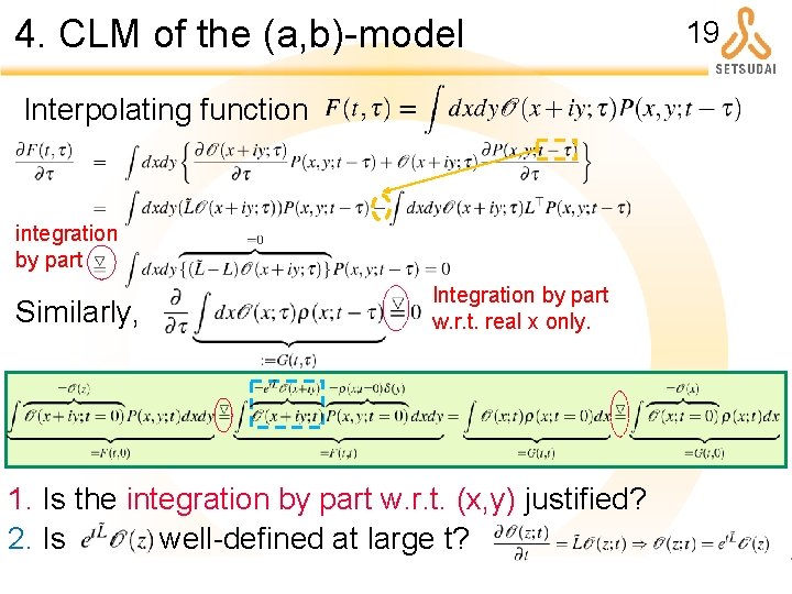
4. CLM of the (a, b)-model Interpolating function integration by part Similarly, Integration by part w. r. t. real x only. 1. Is the integration by part w. r. t. (x, y) justified? 2. Is well-defined at large t? 19

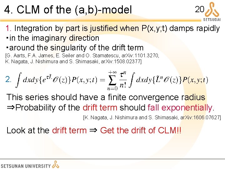
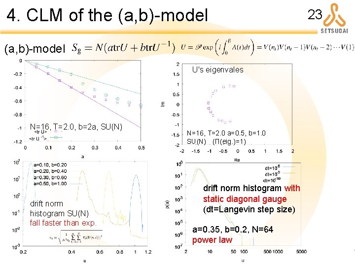
4. CLM of the (a, b)-model 20 1. Integration by part is justified when P(x, y; t) damps rapidly ・in the imaginary direction ・around the singularity of the drift term [G. Aarts, F. A. James, E. Seiler and O. Stamatescu, ar. Xiv: 1101. 3270, K. Nagata, J. Nishimura and S. Shimasaki, ar. Xiv: 1508. 02377] 2. This series should have a finite convergence radius ⇒Probability of the drift term should fall exponentially. [K. Nagata, J. Nishimura and S. Shimasaki, ar. Xiv: 1606. 07627] Look at the drift term ⇒ Get the drift of CLM!!

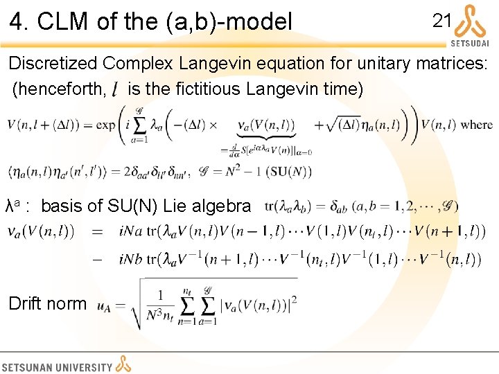
4. CLM of the (a, b)-model 21 Discretized Complex Langevin equation for unitary matrices: (henceforth, is the fictitious Langevin time) λa : basis of SU(N) Lie algebra Drift norm

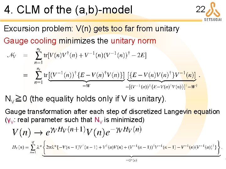
4. CLM of the (a, b)-model 22 Excursion problem: V(n) gets too far from unitary Gauge cooling minimizes the unitary norm NV≧ 0 (the equality holds only if V is unitary). Gauge transformation after each step of discretized Langevin equation (γV: real parameter such that NV is minimized)

4. CLM of the (a, b)-model U's eigenvales N=16, T=2. 0, b=2 a, SU(N) drift norm histogram SU(N) fall faster than exp. N=16, T=2. 0 a=0. 5, b=1. 0 SU(N) 　(Π(eig. )=1) drift norm histogram with static diagonal gauge (dt=Langevin step size) a=0. 35, b=0. 2, N=64 power law 23

5. Summary 24 We have studied the matrix quantum mechanics with a chemical potential ・bosonic model ⇒ GWW-type third-order phase transition (except for very small μ) ・phase diagram of the bosonic/fermionic model Future works: Use of Complex Langevin Method for sign problem: ・Generalization to [P. Basu, K. Jaswin and A. Joseph ar. Xiv: 1802. 10381] ・supersymmetric quantum mechanics [A. Joseph and A. Kumar, ar. Xiv: 1908. 04153]

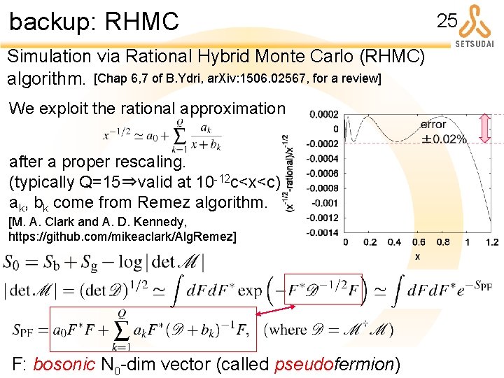
backup: RHMC Simulation via Rational Hybrid Monte Carlo (RHMC) algorithm. [Chap 6, 7 of B. Ydri, ar. Xiv: 1506. 02567, for a review] We exploit the rational approximation after a proper rescaling. (typically Q=15⇒valid at 10 -12 c<x<c) ak, bk come from Remez algorithm. [M. A. Clark and A. D. Kennedy, https: //github. com/mikeaclark/Alg. Remez] F: bosonic N 0 -dim vector (called pseudofermion) 25

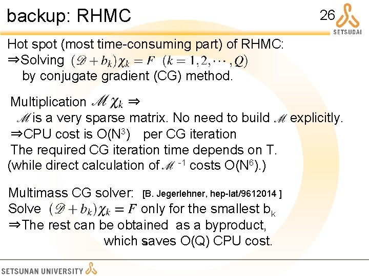
backup: RHMC 26 Hot spot (most time-consuming part) of RHMC: ⇒Solving by conjugate gradient (CG) method. Multiplication ⇒ is a very sparse matrix. No need to build 　 explicitly. ⇒CPU cost is O(N 3)　 per CG iteration The required CG iteration time depends on T. (while direct calculation of -1 costs O(N 6). ) Multimass CG solver: [B. Jegerlehner, hep-lat/9612014 ] Solve only for the smallest b k ⇒The rest can be obtained as a byproduct, which saves O(Q) CPU cost. 26

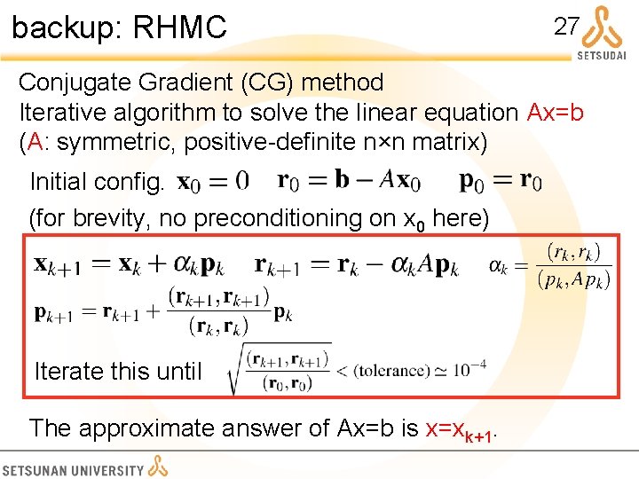
backup: RHMC 27 Conjugate Gradient (CG) method Iterative algorithm to solve the linear equation Ax=b (A: symmetric, positive-definite n×n matrix) Initial config. (for brevity, no preconditioning on x 0 here) Iterate this until The approximate answer of Ax=b is x=xk+1.