Phase Transitions in Random Geometric Graphs with Algorithmic

Phase Transitions in Random Geometric Graphs, with Algorithmic Implications Ashish Goel Stanford University Joint work with Sanatan Rai and Bhaskar Krishnamachari http: //www. stanford. edu/~ashishg@stanford. edu

Geometric Random Graphs • G(n; r) in d-dimensions: – n points uniformly distributed in [0, 1]d – Two points are connected if their Euclidean distance is less than r • Sensor networks can often be modeled as G(n; r) with d=2 – Eg. sensors “sprinkled” from a helicopter over a corn field – The wireless radius corresponds to r • Question: How should n and r be chosen to ensure that G(n; r) has a desirable property (eg. connectivity, 2 connectivity, large cliques) with high probability? ashishg@stanford. edu

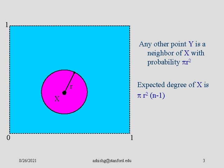
1 Any other point Y is a neighbor of X with probability r 2 Expected degree of X is r 2 (n-1) r X 0 1 8/26/2021 ashishg@stanford. edu 3

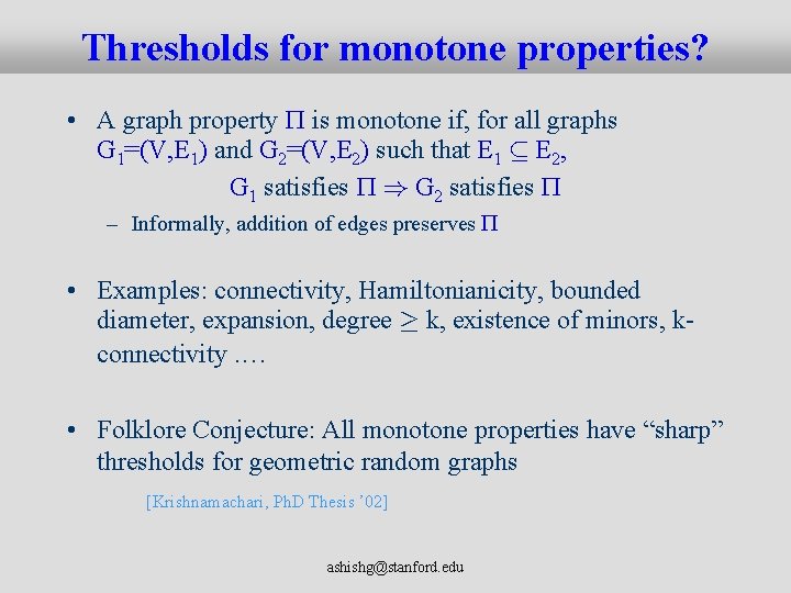
Thresholds for monotone properties? • A graph property is monotone if, for all graphs G 1=(V, E 1) and G 2=(V, E 2) such that E 1 µ E 2, G 1 satisfies ) G 2 satisfies – Informally, addition of edges preserves • Examples: connectivity, Hamiltonianicity, bounded diameter, expansion, degree ¸ k, existence of minors, kconnectivity. … • Folklore Conjecture: All monotone properties have “sharp” thresholds for geometric random graphs [Krishnamachari, Ph. D Thesis ’ 02] ashishg@stanford. edu

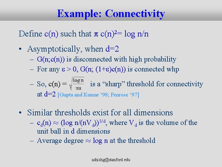
Example: Connectivity Define c(n) such that c(n)2= log n/n • Asymptotically, when d=2 – G(n; c(n)) is disconnected with high probability – For any > 0, G(n; (1+ )c(n)) is connected whp – So, c(n) = is a “sharp” threshold for connectivity at d=2 [Gupta and Kumar ‘ 98; Penrose ‘ 97] • Similar thresholds exist for all dimensions – cd(n) ¼ (log n/(n. Vd))1/d, where Vd is the volume of the unit ball in d dimensions – Average degree ¼ log n at the threshold ashishg@stanford. edu

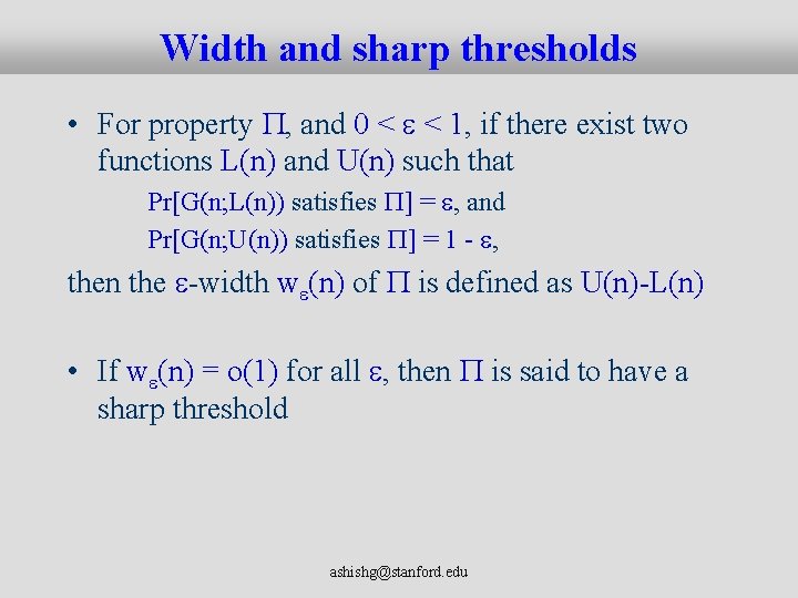
Width and sharp thresholds • For property , and 0 < < 1, if there exist two functions L(n) and U(n) such that Pr[G(n; L(n)) satisfies ] = , and Pr[G(n; U(n)) satisfies ] = 1 - , then the -width w (n) of is defined as U(n)-L(n) • If w (n) = o(1) for all , then is said to have a sharp threshold ashishg@stanford. edu

Example Pr[G(n; r) satisfies ] 1 1 - r 0 Width 8/26/2021 ashishg@stanford. edu 7

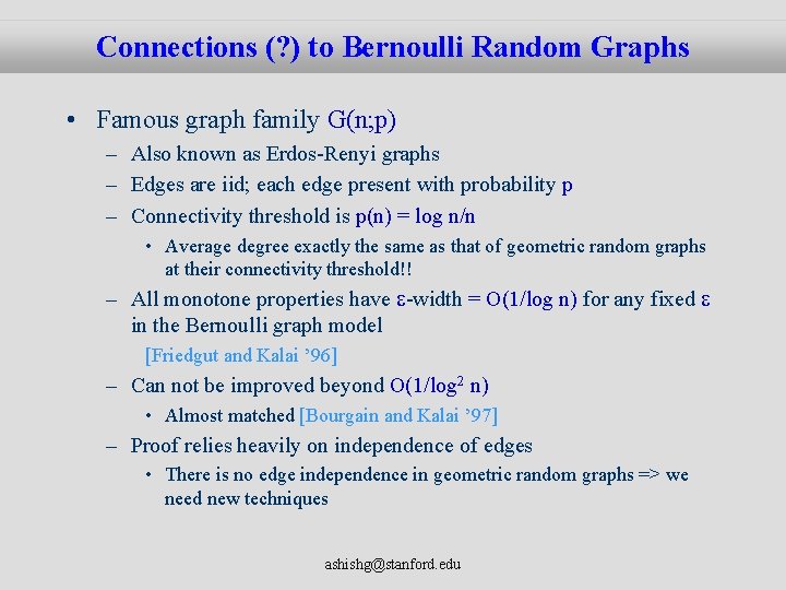
Connections (? ) to Bernoulli Random Graphs • Famous graph family G(n; p) – Also known as Erdos-Renyi graphs – Edges are iid; each edge present with probability p – Connectivity threshold is p(n) = log n/n • Average degree exactly the same as that of geometric random graphs at their connectivity threshold!! – All monotone properties have -width = O(1/log n) for any fixed in the Bernoulli graph model [Friedgut and Kalai ’ 96] – Can not be improved beyond O(1/log 2 n) • Almost matched [Bourgain and Kalai ’ 97] – Proof relies heavily on independence of edges • There is no edge independence in geometric random graphs => we need new techniques ashishg@stanford. edu

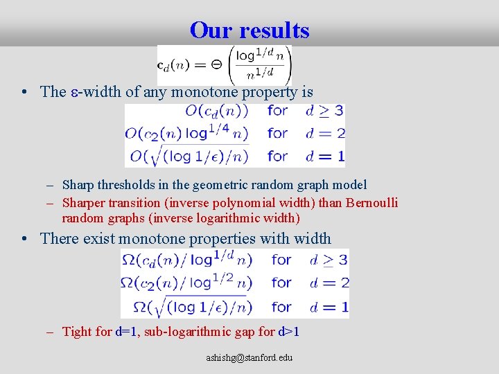
Our results • The -width of any monotone property is – Sharp thresholds in the geometric random graph model – Sharper transition (inverse polynomial width) than Bernoulli random graphs (inverse logarithmic width) • There exist monotone properties with width – Tight for d=1, sub-logarithmic gap for d>1 ashishg@stanford. edu

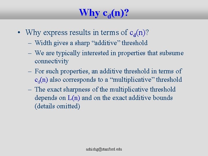
Why cd(n)? • Why express results in terms of cd(n)? – Width gives a sharp “additive” threshold – We are typically interested in properties that subsume connectivity – For such properties, an additive threshold in terms of cd(n) also corresponds to a “multiplicative” threshold – The exact sharpness of the multiplicative threshold depends on L(n) and on the exact additive bounds (details omitted) ashishg@stanford. edu

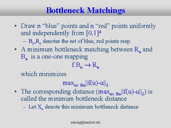
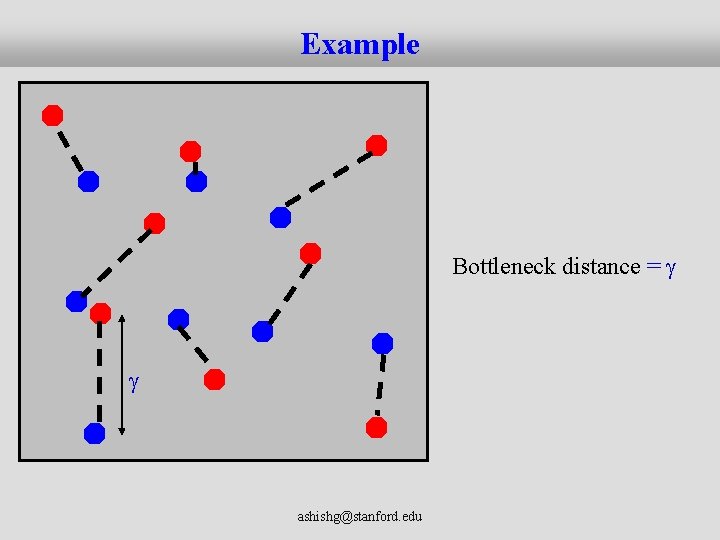
Bottleneck Matchings • Draw n “blue” points and n “red” points uniformly and independently from [0, 1]d – Bn, Rn denotes the set of blue, red points resp. • A minimum bottleneck matching between Rn and Bn is a one-one mapping f: Bn ! Rn which minimizes maxu 2 Bn||f(u)-u||2 • The corresponding distance (maxu 2 Bn||f(u)-u||2) is called the minimum bottleneck distance – Let Xn denote this minimum bottleneck distance ashishg@stanford. edu

Example Bottleneck distance = ashishg@stanford. edu

Bottleneck Matchings and Width Theorem: If Pr[Xn > ] · p then the sqrt(p)-width of any monotone property is at most 2 Implication: Can analyze just one quantity, Xn, as opposed to all monotone properties (in particular, can provide simulation based evidence) Proof: Let be any monotone property Let = sqrt(p) Choose L(n) such that Pr[G(n; L(n) satisfies ] = Define U(n) = L(n) + 2 Draw two random graphs GL and GU (independently) from G(n; L(n)) and G(n; U(n)), resp. – Let Bn, Rn denote the set of points in GL, GU resp. – – ashishg@stanford. edu

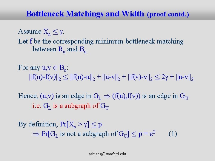
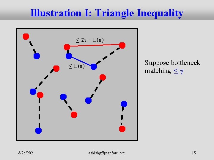
Bottleneck Matchings and Width (proof contd. ) Assume Xn · . Let f be the corresponding minimum bottleneck matching between Rn and Bn. For any u, v 2 Bn: ||f(u)-f(v)||2 · ||f(u)-u||2 + ||u-v||2 + ||f(v)-v||2 · 2 + ||u-v||2 Hence, (u, v) is an edge in GL ) (f(u), f(v)) is an edge in GU i. e. GL is a subgraph of GU By definition, Pr[Xn > ] · p ) Pr[GL is not a subgraph of GU] · p = 2 ashishg@stanford. edu (1)

Illustration I: Triangle Inequality · 2 + L(n) Suppose bottleneck matching · · L(n) 8/26/2021 ashishg@stanford. edu 15

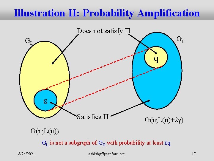
Bottleneck Matchings and Width (proof contd. ) Pr[GL is not a subgraph of GU] · p = 2 (1) Let q = Pr[GU does not satisfy ] is monotone, Pr[GL satisfies ] = , ) Pr[GL is not a subgraph of GU] ¸ ¢q Combining (1) and (2), we get ¢q · p i. e. q · Therefore, Pr[GU satisfies ] ¸ 1 - i. e. the -width of is at most U(n) – L(n) = 2 Done! ashishg@stanford. edu (2)

Illustration II: Probability Amplification Does not satisfy GU GL q Satisfies G(n; L(n)+2 ) G(n; L(n)) GL is not a subgraph of GU with probability at least q 8/26/2021 ashishg@stanford. edu 17

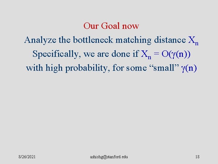
Our Goal now Analyze the bottleneck matching distance Xn Specifically, we are done if Xn = O( (n)) with high probability, for some “small” (n) 8/26/2021 ashishg@stanford. edu 18

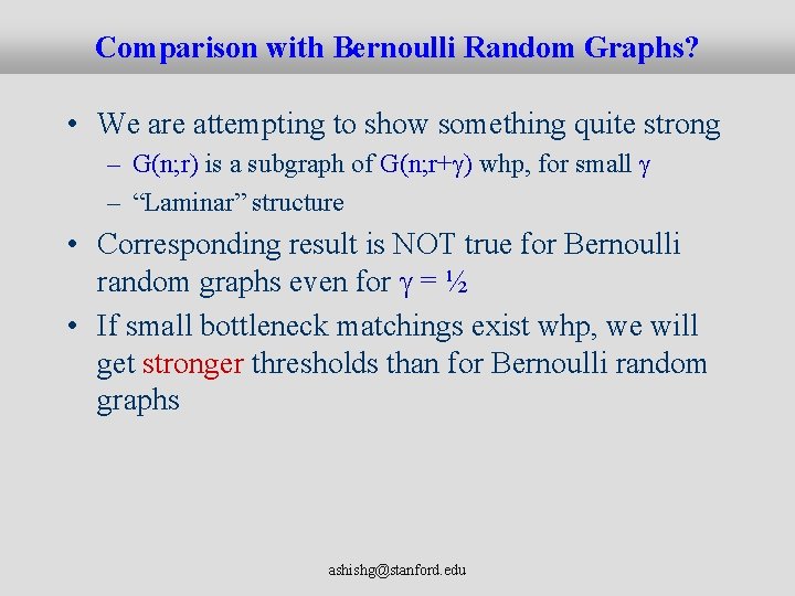
Comparison with Bernoulli Random Graphs? • We are attempting to show something quite strong – G(n; r) is a subgraph of G(n; r+ ) whp, for small – “Laminar” structure • Corresponding result is NOT true for Bernoulli random graphs even for = ½ • If small bottleneck matchings exist whp, we will get stronger thresholds than for Bernoulli random graphs ashishg@stanford. edu

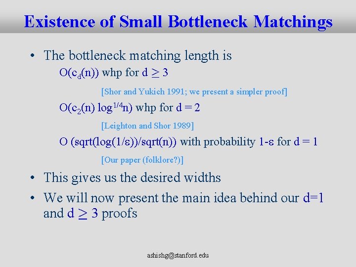
Existence of Small Bottleneck Matchings • The bottleneck matching length is O(cd(n)) whp for d ¸ 3 [Shor and Yukich 1991; we present a simpler proof] O(c 2(n) log 1/4 n) whp for d = 2 [Leighton and Shor 1989] O (sqrt(log(1/ ))/sqrt(n)) with probability 1 - for d = 1 [Our paper (folklore? )] • This gives us the desired widths • We will now present the main idea behind our d=1 and d ¸ 3 proofs ashishg@stanford. edu

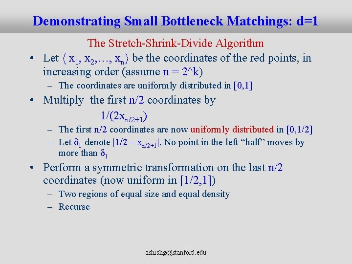
Demonstrating Small Bottleneck Matchings: d=1 The Stretch-Shrink-Divide Algorithm • Let h x 1, x 2, …, xni be the coordinates of the red points, in increasing order (assume n = 2^k) – The coordinates are uniformly distributed in [0, 1] • Multiply the first n/2 coordinates by 1/(2 xn/2+1) – The first n/2 coordinates are now uniformly distributed in [0, 1/2] – Let d 1 denote |1/2 – xn/2+1|. No point in the left “half” moves by more than d 1 • Perform a symmetric transformation on the last n/2 coordinates (now uniform in [1/2, 1]) – Two regions of equal size and equal density – Recurse ashishg@stanford. edu

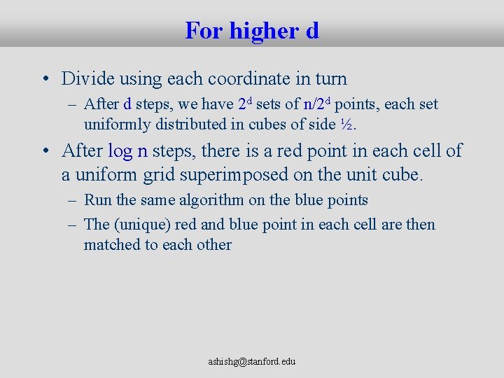
For higher d • Divide using each coordinate in turn – After d steps, we have 2 d sets of n/2 d points, each set uniformly distributed in cubes of side ½. • After log n steps, there is a red point in each cell of a uniform grid superimposed on the unit cube. – Run the same algorithm on the blue points – The (unique) red and blue point in each cell are then matched to each other ashishg@stanford. edu

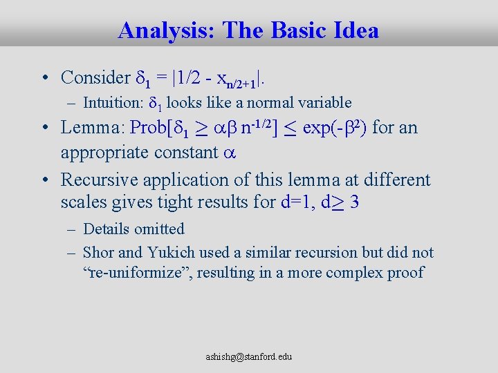
Analysis: The Basic Idea • Consider d 1 = |1/2 - xn/2+1|. – Intuition: d 1 looks like a normal variable • Lemma: Prob[d 1 ¸ ab n-1/2] · exp(-b 2) for an appropriate constant a • Recursive application of this lemma at different scales gives tight results for d=1, d¸ 3 – Details omitted – Shor and Yukich used a similar recursion but did not “re-uniformize”, resulting in a more complex proof ashishg@stanford. edu

Lower bound examples • For d=1, the property = {G: 8 v 2 V(G), degree(v) ¸ |V(G)|/4} has width W(sqrt(log 1/ )/sqrt(n)) – Basic idea: Just the two endpoints on the line are interesting for the purpose of finding the minimum degree • For d¸ 2, the property = {G is a clique}has width W(1/n 1/d) • Open problem: plug the gap in the upper/lower bounds on the width for d ¸ 2 – Also, all our lower bound examples undergo phase transitions at r = Q(1). Is there something interesting and different in the region where r is of the order of the connectivity threshold? ashishg@stanford. edu

Implications – Mixing Time Recent result: Fastest mixing Markov chain defined on G(n; r) has mixing time Q(r-2 log n) for large enough r [Boyd, Ghosh, Prabhakar, Shah ‘ 05] Alternate proof: – GRID(n; r): n points are laid on a grid in [0, 1]2 and two points are connected if they are within distance r. – Fastest mixing time of GRID(n; r) = Q(r-2 log n) [Trivial] – G(n; r) is a super-graph of GRID(n; r-d) and a sub-graph of G(n; r+d) whp for small enough d [Our result] ) Fastest mixing time of G(n; r) is Q(r-2 log n) whp ashishg@stanford. edu

Implications – Spectra Our techniques can be extended to show that the spectrum of random geometric graphs converges to the spectrum of the grid graph. [Rai ’ 05] ashishg@stanford. edu

Implications – Coverage • Coverage: Any point in the unit square must be within a distance r from one of the n sensors – Known: there is a sharp threshold in r [Shakkottai, Srikant, Shroff ’ 04] – Coverage is NOT a graph property, so it does not fall within our framework – But the laminar structure in our proof implies a sharp threshold for coverage as well (weaker than the sharpest known) ashishg@stanford. edu

Conclusions • Monotone properties in G(n; r) have sharp thresholds – Much sharper than for Bernoulli Random Graphs • Much stronger too: Random geometric graphs exhibit a laminar structure – Useful for recovering several known results/proving new ones – Randomness is often a red-herring since the deterministic grid often yields asymptotically tight upper and lower bounds • Open problem: Does laminarity imply anything about throughput (via separators)? ashishg@stanford. edu