Phantom Works Mathematics Computing Technology Real Options and

Phantom Works Mathematics & Computing Technology Real Options and Mean-Reverting Prices Gregory F. Robel Mathematics & Engineering Analysis July 14, 2001 gregory. f. robel@boeing. com

Acknowledgements Phantom Works Mathematics & Computing Technology I would like to thank several colleagues for useful discussions, including Dr. Stuart Anderson, Dr. Mike Epton and Dr. Roman Fresnedo of The Boeing Company; and Dr. Dan Calistrate and Professor Gordon Sick of The University of Calgary. The usual disclaimer applies. 2

Outline Phantom Works Mathematics & Computing Technology • • Standard capital budgeting paradigm Real option extension of standard paradigm Mc. Donald-Siegel model Survey and critique of some proposed models of meanreverting prices Specification of a “new, ” more appropriate model Analytical solution of some option problems for the “new” model, and some comparative statics Remarks on numerical approaches for more complex problems Conclusion 3

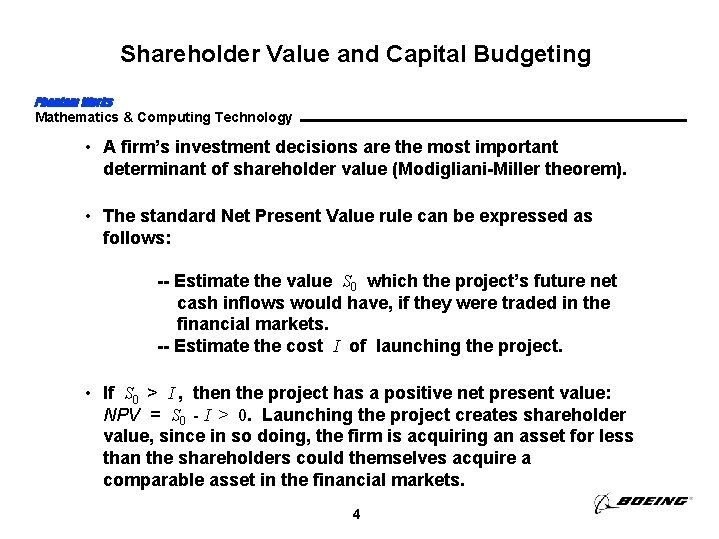
Shareholder Value and Capital Budgeting Phantom Works Mathematics & Computing Technology • A firm’s investment decisions are the most important determinant of shareholder value (Modigliani-Miller theorem). • The standard Net Present Value rule can be expressed as follows: -- Estimate the value S 0 which the project’s future net cash inflows would have, if they were traded in the financial markets. -- Estimate the cost I of launching the project. • If S 0 > I , then the project has a positive net present value: NPV = S 0 - I > 0. Launching the project creates shareholder value, since in so doing, the firm is acquiring an asset for less than the shareholders could themselves acquire a comparable asset in the financial markets. 4

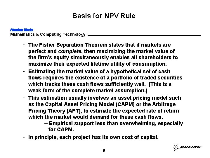
Basis for NPV Rule Phantom Works Mathematics & Computing Technology • The Fisher Separation Theorem states that if markets are perfect and complete, then maximizing the market value of the firm’s equity simultaneously enables all shareholders to maximize their expected lifetime utility of consumption. • Estimating the market value of a hypothetical set of cash flows requires the existence of a portfolio of traded securities which tracks these cash flows sufficiently well. (This is a weak form of the complete market assumption. ) • This estimation usually involves an asset pricing model such as the Capital Asset Pricing Model (CAPM) or the Arbitrage Pricing Theory (APT), to estimate the expected rate of return which the market would demand for these cash flows. -- Empirical support less than overwhelming, especially for CAPM. • In principle, each project has its own cost of capital. 5

Critique of NPV Rule Phantom Works Mathematics & Computing Technology • Correct, as far as it goes. • Implicit assumptions: -- Project has a directly associated stream of future net cash inflows -- Decision must be made now or never -- Management strategy fixed in advance -- Similar to evaluating stocks or bonds 6

Real Options Phantom Works Mathematics & Computing Technology • Many projects create future opportunities, which may be a significant, or even the sole, source of value. • These opportunities are analogous to financial options. • The term real options has been coined to refer to a firm’s discretionary opportunities involving real assets. • Discounted cash flow methods fail for the evaluation of options. • Financial economists have recognized the analogy between real and financial options. • The same assumptions which justify the use of discounted cash flow methods for evaluating a project also justify the use of an option pricing model for evaluating options associated with the project. Reference: [Co. A] 7

Types of Options Phantom Works Mathematics & Computing Technology • In general, an option is a financial contract which gives its holder the right, but not the obligation, to buy or sell another, underlying asset, at a specified price, on or until a specified expiration date. • An option to buy is a call option. • An option to sell is a put option. • An option with an infinite expiration date is said to be perpetual. • An option which can be exercised only on its expiration date is said to be European. • An option which can be exercised at any time up until and including its expiration date is said to be American. 8

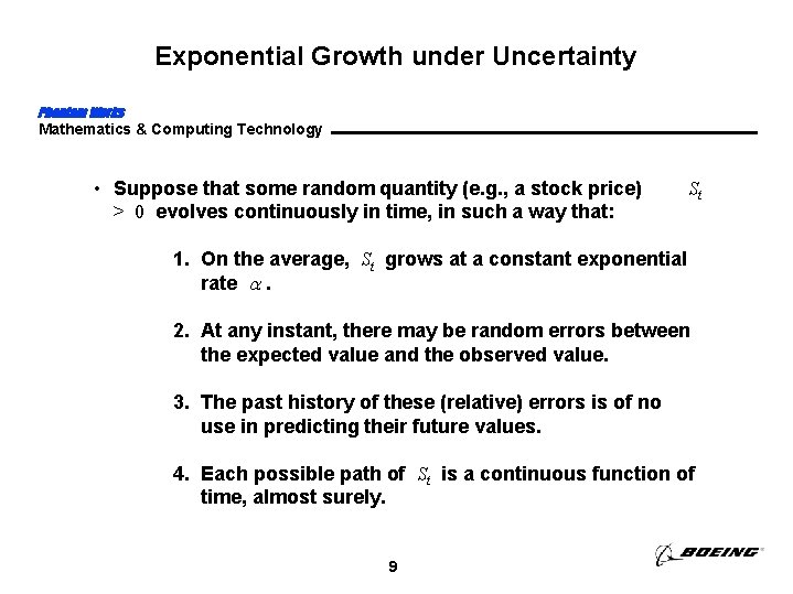
Exponential Growth under Uncertainty Phantom Works Mathematics & Computing Technology • Suppose that some random quantity (e. g. , a stock price) > 0 evolves continuously in time, in such a way that: St 1. On the average, St grows at a constant exponential rate . 2. At any instant, there may be random errors between the expected value and the observed value. 3. The past history of these (relative) errors is of no use in predicting their future values. 4. Each possible path of St is a continuous function of time, almost surely. 9

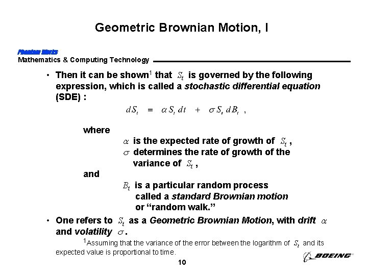
Geometric Brownian Motion, I Phantom Works Mathematics & Computing Technology • Then it can be shown 1 that St is governed by the following expression, which is called a stochastic differential equation (SDE) : where and is the expected rate of growth of St , determines the rate of growth of the variance of St , Bt is a particular random process called a standard Brownian motion or “random walk. ” • One refers to St as a Geometric Brownian Motion, with drift and volatility . 1 Assuming that the variance of the error between the logarithm of S and its t expected value is proportional to time. 10

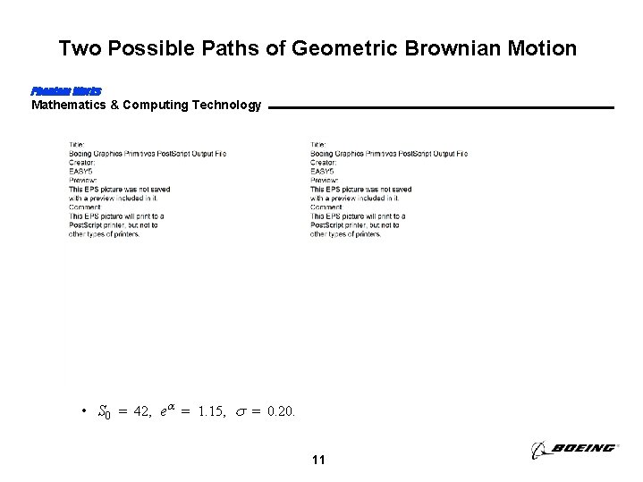
Two Possible Paths of Geometric Brownian Motion Phantom Works Mathematics & Computing Technology • S 0 = 42, e = 1. 15, = 0. 20. 11

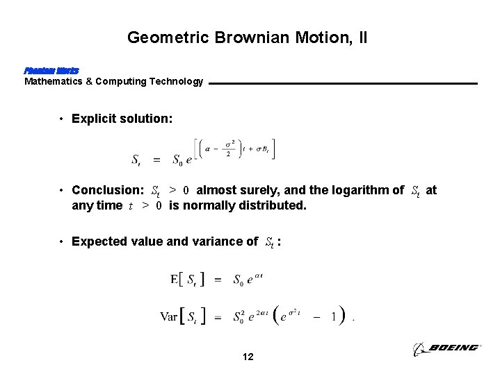
Geometric Brownian Motion, II Phantom Works Mathematics & Computing Technology • Explicit solution: • Conclusion: St > 0 almost surely, and the logarithm of St at any time t > 0 is normally distributed. • Expected value and variance of St : 12

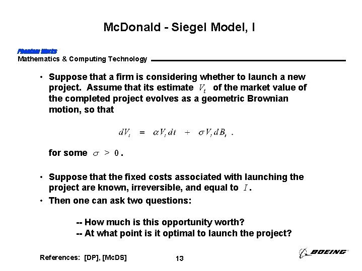
Mc. Donald - Siegel Model, I Phantom Works Mathematics & Computing Technology • Suppose that a firm is considering whether to launch a new project. Assume that its estimate Vt of the market value of the completed project evolves as a geometric Brownian motion, so that for some > 0. • Suppose that the fixed costs associated with launching the project are known, irreversible, and equal to I. • Then one can ask two questions: -- How much is this opportunity worth? -- At what point is it optimal to launch the project? References: [DP], [Mc. DS] 13

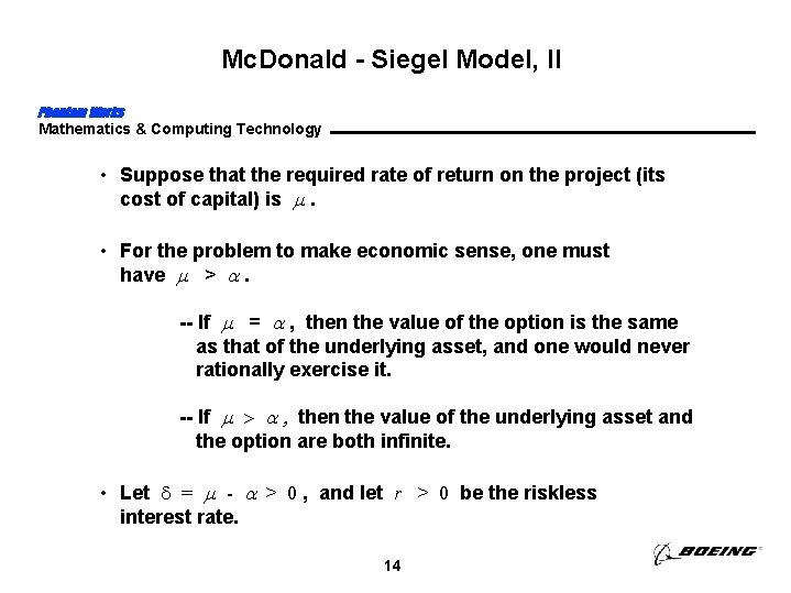
Mc. Donald - Siegel Model, II Phantom Works Mathematics & Computing Technology • Suppose that the required rate of return on the project (its cost of capital) is . • For the problem to make economic sense, one must have > . -- If = , then the value of the option is the same as that of the underlying asset, and one would never rationally exercise it. -- If , then the value of the underlying asset and the option are both infinite. • Let d = - > 0 , and let r > 0 be the riskless interest rate. 14

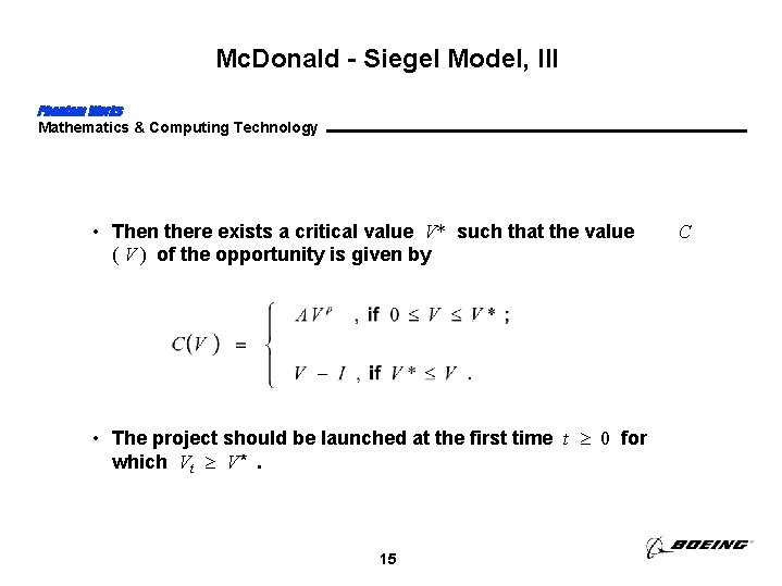
Mc. Donald - Siegel Model, III Phantom Works Mathematics & Computing Technology • Then there exists a critical value V* such that the value ( V ) of the opportunity is given by • The project should be launched at the first time t 0 for which Vt V*. 15 C

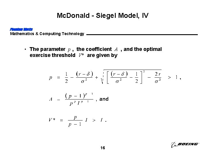
Mc. Donald - Siegel Model, IV Phantom Works Mathematics & Computing Technology • The parameter p , the coefficient A , and the optimal exercise threshold V* are given by 16

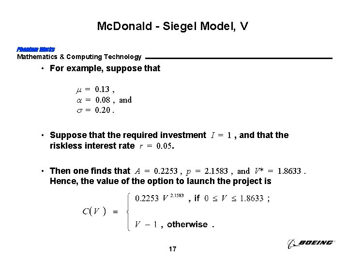
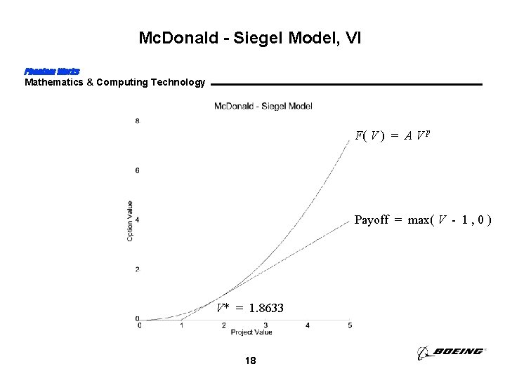
Mc. Donald - Siegel Model, V Phantom Works Mathematics & Computing Technology • For example, suppose that = 0. 13 , = 0. 08 , and = 0. 20. • Suppose that the required investment I = 1 , and that the riskless interest rate r = 0. 05. • Then one finds that A = 0. 2253 , p = 2. 1583 , and V* = 1. 8633. Hence, the value of the option to launch the project is 17

Mc. Donald - Siegel Model, VI Phantom Works Mathematics & Computing Technology F( V ) = A V p Payoff = max( V - 1 , 0 ) V* = 1. 8633 18

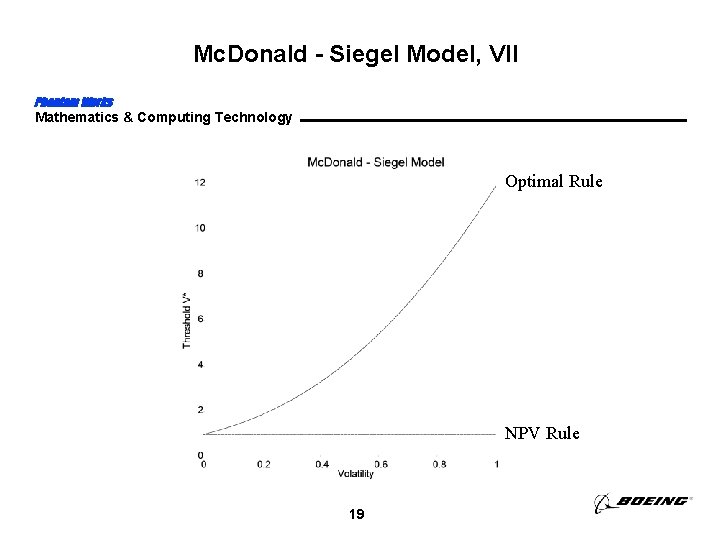
Mc. Donald - Siegel Model, VII Phantom Works Mathematics & Computing Technology Optimal Rule NPV Rule 19

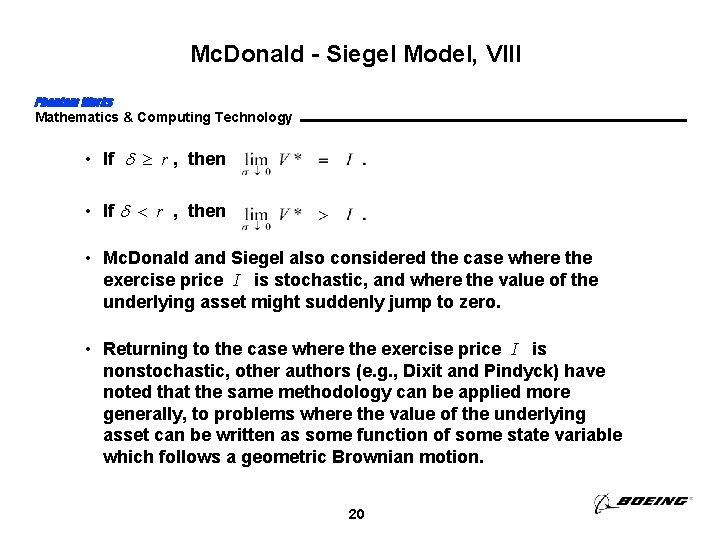
Mc. Donald - Siegel Model, VIII Phantom Works Mathematics & Computing Technology • If r , then • Mc. Donald and Siegel also considered the case where the exercise price I is stochastic, and where the value of the underlying asset might suddenly jump to zero. • Returning to the case where the exercise price I is nonstochastic, other authors (e. g. , Dixit and Pindyck) have noted that the same methodology can be applied more generally, to problems where the value of the underlying asset can be written as some function of some state variable which follows a geometric Brownian motion. 20

Motivation for Mean-Reverting Prices Phantom Works Mathematics & Computing Technology • The “workhorse” stochastic process for much of the early work on real options is geometric Brownian motion. • This is a natural model for exponential growth (or decay) under uncertainty. • Consider a real option where the underlying state variable is the price of some input or output. • One might argue that the price may be subject to random shocks, but that in the long run, competitive pressures will ensure that it tends to revert to some sustainable level. 21

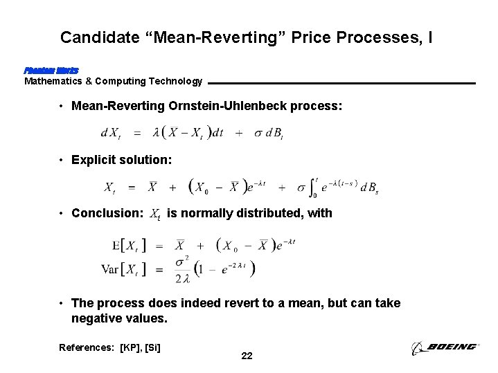
Candidate “Mean-Reverting” Price Processes, I Phantom Works Mathematics & Computing Technology • Mean-Reverting Ornstein-Uhlenbeck process: • Explicit solution: • Conclusion: Xt is normally distributed, with • The process does indeed revert to a mean, but can take negative values. References: [KP], [Si] 22

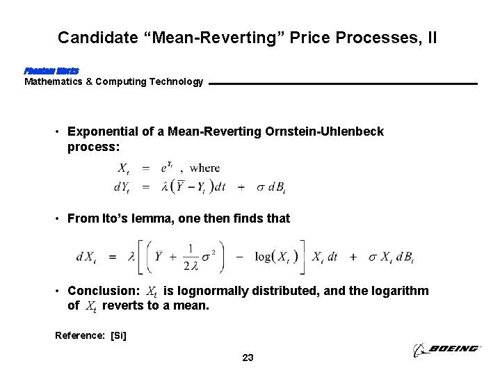
Candidate “Mean-Reverting” Price Processes, II Phantom Works Mathematics & Computing Technology • Exponential of a Mean-Reverting Ornstein-Uhlenbeck process: • From Ito’s lemma, one then finds that • Conclusion: Xt is lognormally distributed, and the logarithm of Xt reverts to a mean. Reference: [Si] 23

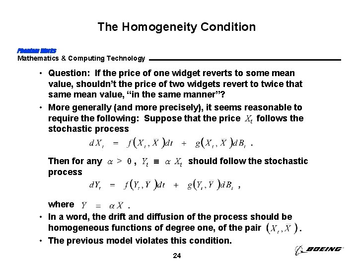
The Homogeneity Condition Phantom Works Mathematics & Computing Technology • Question: If the price of one widget reverts to some mean value, shouldn’t the price of two widgets revert to twice that same mean value, “in the same manner”? • More generally (and more precisely), it seems reasonable to require the following: Suppose that the price Xt follows the stochastic process Then for any > 0 , Yt Xt should follow the stochastic process where • In a word, the drift and diffusion of the process should be homogeneous functions of degree one, of the pair • The previous model violates this condition. 24

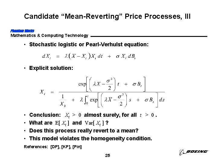
Candidate “Mean-Reverting” Price Processes, III Phantom Works Mathematics & Computing Technology • Stochastic logistic or Pearl-Verhulst equation: • Explicit solution: • • Conclusion: Xt > 0 almost surely, for all t > 0. What are E[ Xt ] and Var[ Xt ] ? Does this process really revert to a mean? This model violates the homogeneity condition. References: [DP], [KP], [Pin] 25

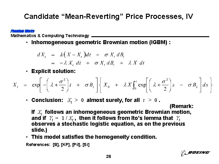
Candidate “Mean-Reverting” Price Processes, IV Phantom Works Mathematics & Computing Technology • Inhomogeneous geometric Brownian motion (IGBM) : • Explicit solution: • Conclusion: Xt > 0 almost surely, for all t > 0. (Remark: If Xt follows an inhomogeneous geometric Brownian motion, and if Yt = 1 / Xt , then it follows from Ito’s lemma that Yt observes a stochastic logistic equation, as on the previous slide. ) • This model satisfies the homogeneity condition. References: [B], [KP], [Pil], [Si] 26

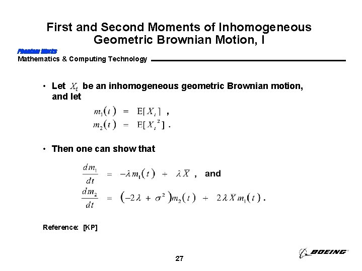
First and Second Moments of Inhomogeneous Geometric Brownian Motion, I Phantom Works Mathematics & Computing Technology • Let Xt be an inhomogeneous geometric Brownian motion, and let • Then one can show that Reference: [KP] 27

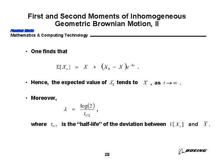
First and Second Moments of Inhomogeneous Geometric Brownian Motion, II Phantom Works Mathematics & Computing Technology • One finds that • Hence, the expected value of Xt tends to • Moreover, where is the “half-life” of the deviation between 28

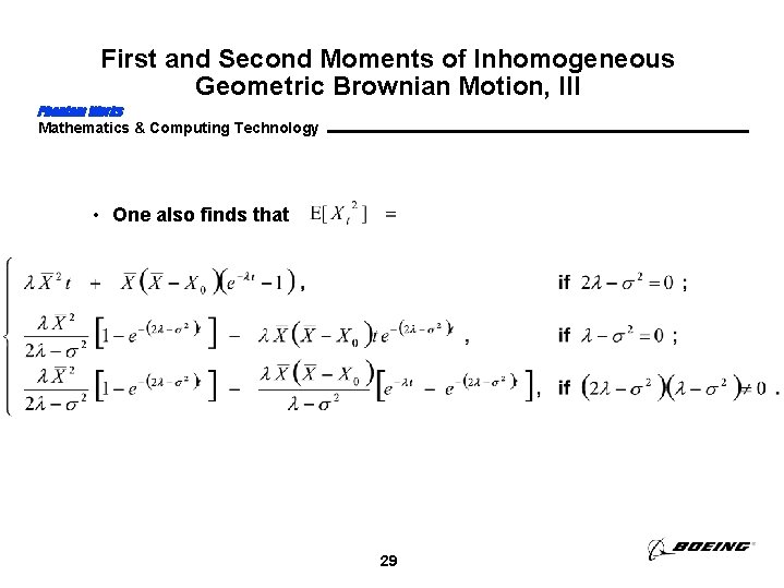
First and Second Moments of Inhomogeneous Geometric Brownian Motion, III Phantom Works Mathematics & Computing Technology • One also finds that 29

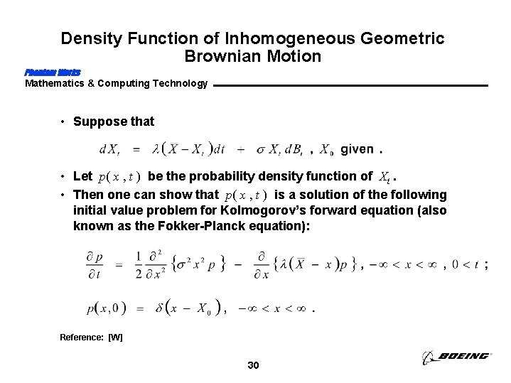
Density Function of Inhomogeneous Geometric Brownian Motion Phantom Works Mathematics & Computing Technology • Suppose that • Let p( x , t ) be the probability density function of Xt. • Then one can show that p( x , t ) is a solution of the following initial value problem for Kolmogorov’s forward equation (also known as the Fokker-Planck equation): Reference: [W] 30

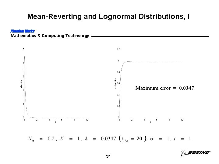
Mean-Reverting and Lognormal Distributions, I Phantom Works Mathematics & Computing Technology Maximum error = 0. 0347 31

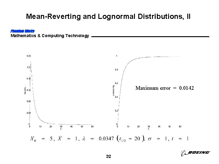
Mean-Reverting and Lognormal Distributions, II Phantom Works Mathematics & Computing Technology Maximum error = 0. 0142 32

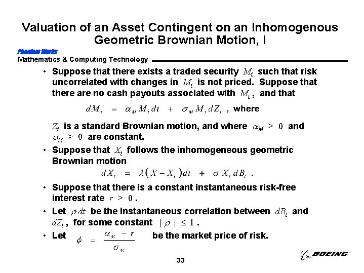
Valuation of an Asset Contingent on an Inhomogenous Geometric Brownian Motion, I Phantom Works Mathematics & Computing Technology • Suppose that there exists a traded security Mt such that risk uncorrelated with changes in Mt is not priced. Suppose that there are no cash payouts associated with Mt , and that Zt is a standard Brownian motion, and where M > 0 and M > 0 are constant. • Suppose that Xt follows the inhomogeneous geometric Brownian motion • Suppose that there is a constant instantaneous risk-free interest rate r > 0. • Let dt be the instantaneous correlation between d. Bt and d. Zt , for some constant | | 1. • Let be the market price of risk. 33

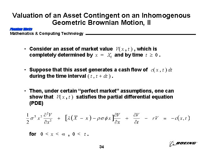
Valuation of an Asset Contingent on an Inhomogenous Geometric Brownian Motion, II Phantom Works Mathematics & Computing Technology • Consider an asset of market value V( x , t ) , which is completely determined by x = Xt and by time t 0. • Suppose that this asset generates a cash flow of c( x , t ) dt during the time interval ( t , t + dt ). • Then, under certain “perfect market” assumptions, one can show that V( x , t ) satisfies the partial differential equation (PDE) for 0 < x < , 0 < t. 34

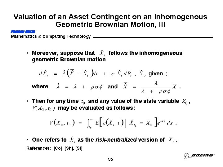
Valuation of an Asset Contingent on an Inhomogenous Geometric Brownian Motion, III Phantom Works Mathematics & Computing Technology • Moreover, suppose that follows the inhomogeneous geometric Brownian motion where • Then for any time t 0 and any value of the state variable X 0 , V( X 0 , t 0 ) may be evaluated as follows: • One refers to as the risk-neutralized version of References: [Co], [Sh], [Si] 35 .

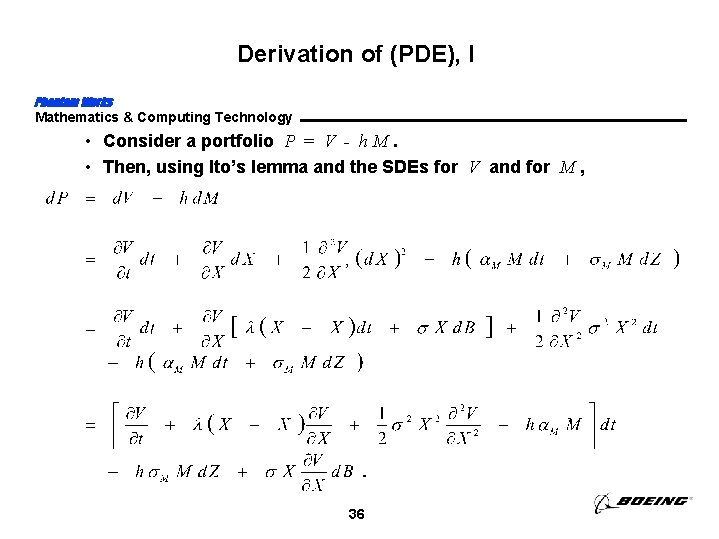
Derivation of (PDE), I Phantom Works Mathematics & Computing Technology • Consider a portfolio P = V - h M. • Then, using Ito’s lemma and the SDEs for V and for M , 36

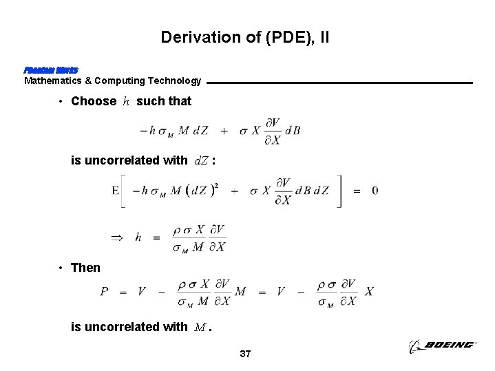
Derivation of (PDE), II Phantom Works Mathematics & Computing Technology • Choose h such that is uncorrelated with d. Z : • Then is uncorrelated with M. 37

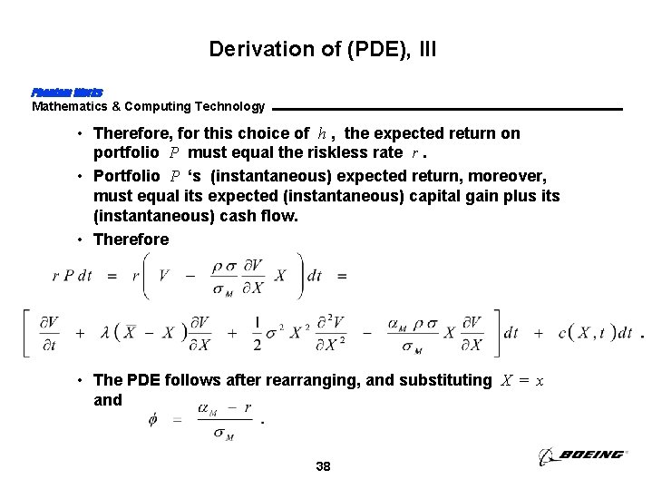
Derivation of (PDE), III Phantom Works Mathematics & Computing Technology • Therefore, for this choice of h , the expected return on portfolio P must equal the riskless rate r. • Portfolio P ‘s (instantaneous) expected return, moreover, must equal its expected (instantaneous) capital gain plus its (instantaneous) cash flow. • Therefore • The PDE follows after rearranging, and substituting X = x and 38

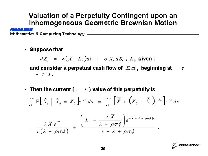
Valuation of a Perpetuity Contingent upon an Inhomogeneous Geometric Brownian Motion Phantom Works Mathematics & Computing Technology • Suppose that and consider a perpetual cash flow of Xt dt , beginning at = 0. • Then the current ( t = 0 ) value of this perpetuity is 39 t

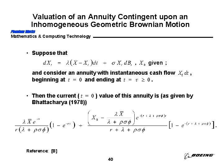
Valuation of an Annuity Contingent upon an Inhomogeneous Geometric Brownian Motion Phantom Works Mathematics & Computing Technology • Suppose that and consider an annuity with instantaneous cash flow Xt dt , beginning at t = 0 and ending at t = 0. • Then the current ( t = 0 ) value of this annuity is (as given by Bhattacharya (1978)) Reference: [B] 40

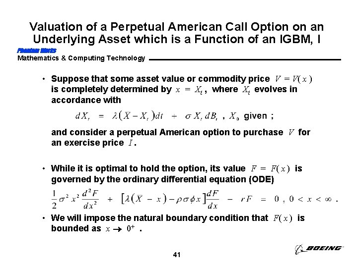
Valuation of a Perpetual American Call Option on an Underlying Asset which is a Function of an IGBM, I Phantom Works Mathematics & Computing Technology • Suppose that some asset value or commodity price V = V( x ) is completely determined by x = Xt , where Xt evolves in accordance with and consider a perpetual American option to purchase V for an exercise price I. • While it is optimal to hold the option, its value F = F( x ) is governed by the ordinary differential equation (ODE) • We will impose the natural boundary condition that F( x ) is bounded as x 0+. 41

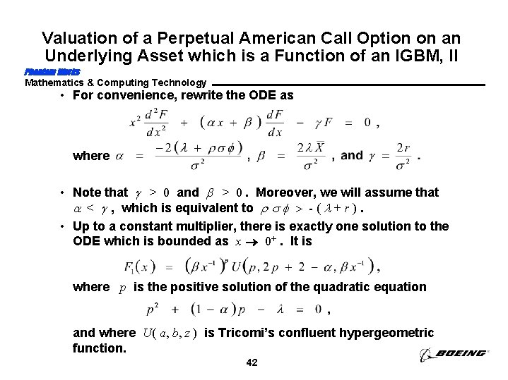
Valuation of a Perpetual American Call Option on an Underlying Asset which is a Function of an IGBM, II Phantom Works Mathematics & Computing Technology • For convenience, rewrite the ODE as where • Note that > 0 and b > 0. Moreover, we will assume that < , which is equivalent to - ( + r ). • Up to a constant multiplier, there is exactly one solution to the ODE which is bounded as x 0+. It is where p is the positive solution of the quadratic equation and where U( a, b, z ) is Tricomi’s confluent hypergeometric function. 42

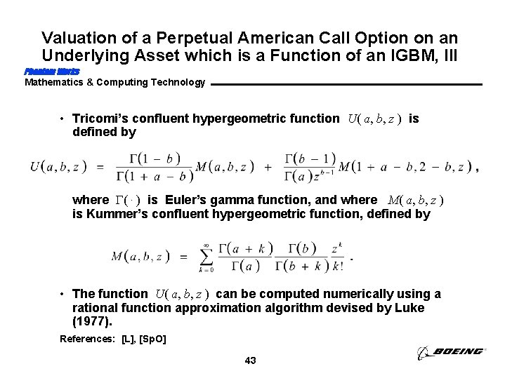
Valuation of a Perpetual American Call Option on an Underlying Asset which is a Function of an IGBM, III Phantom Works Mathematics & Computing Technology • Tricomi’s confluent hypergeometric function U( a, b, z ) is defined by where (. ) is Euler’s gamma function, and where M( a, b, z ) is Kummer’s confluent hypergeometric function, defined by • The function U( a, b, z ) can be computed numerically using a rational function approximation algorithm devised by Luke (1977). References: [L], [Sp. O] 43

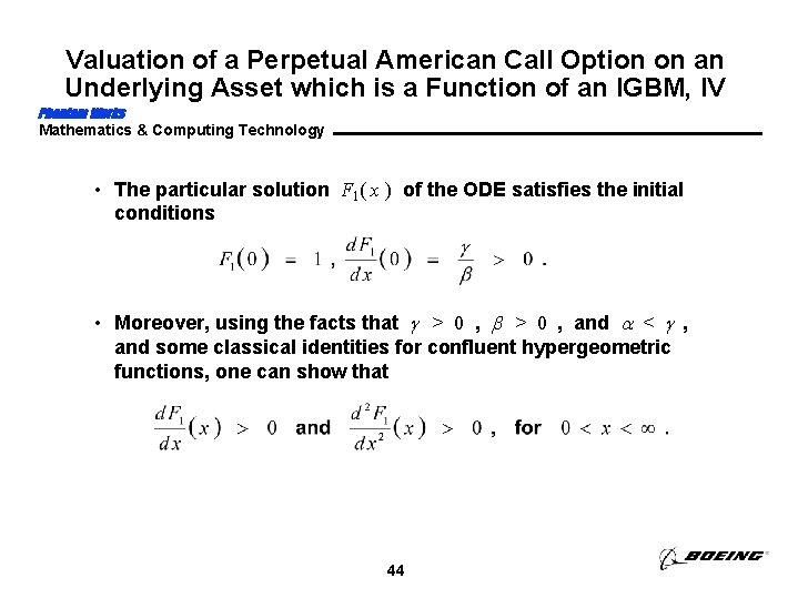
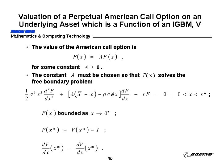
Valuation of a Perpetual American Call Option on an Underlying Asset which is a Function of an IGBM, IV Phantom Works Mathematics & Computing Technology • The particular solution F 1( x ) of the ODE satisfies the initial conditions • Moreover, using the facts that > 0 , b > 0 , and < , and some classical identities for confluent hypergeometric functions, one can show that 44

Valuation of a Perpetual American Call Option on an Underlying Asset which is a Function of an IGBM, V Phantom Works Mathematics & Computing Technology • The value of the American call option is for some constant A > 0. • The constant A must be chosen so that F( x ) solves the free boundary problem 45

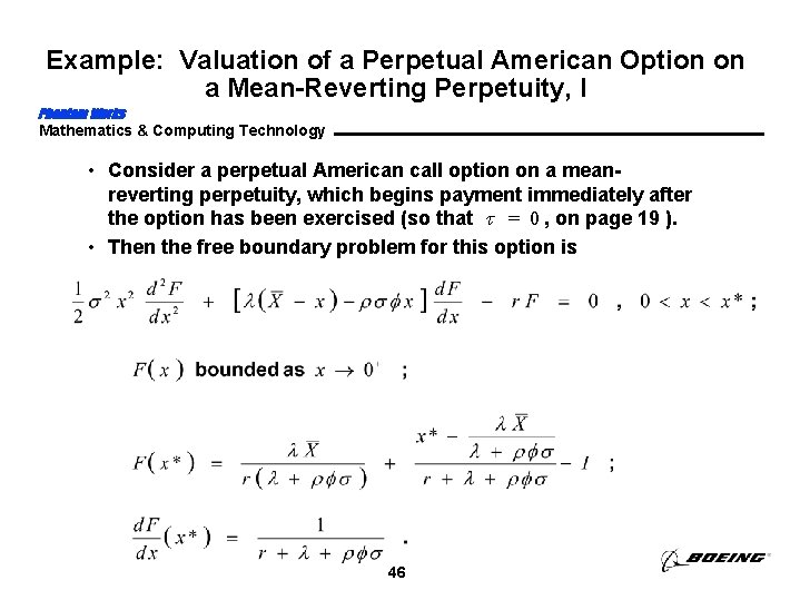
Example: Valuation of a Perpetual American Option on a Mean-Reverting Perpetuity, I Phantom Works Mathematics & Computing Technology • Consider a perpetual American call option on a meanreverting perpetuity, which begins payment immediately after the option has been exercised (so that = 0 , on page 19 ). • Then the free boundary problem for this option is 46

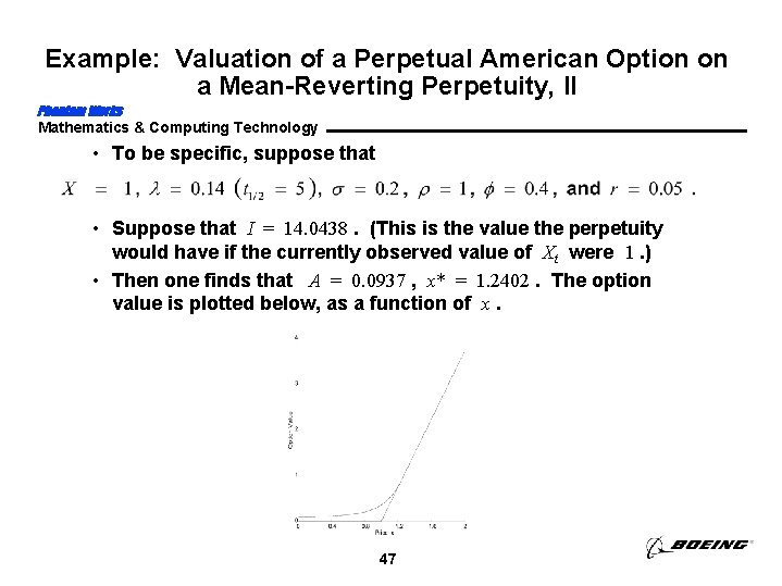
Example: Valuation of a Perpetual American Option on a Mean-Reverting Perpetuity, II Phantom Works Mathematics & Computing Technology • To be specific, suppose that • Suppose that I = 14. 0438. (This is the value the perpetuity would have if the currently observed value of Xt were 1. ) • Then one finds that A = 0. 0937 , x* = 1. 2402. The option value is plotted below, as a function of x. 47

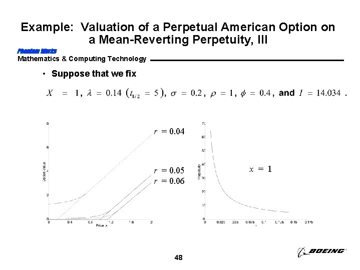
Example: Valuation of a Perpetual American Option on a Mean-Reverting Perpetuity, III Phantom Works Mathematics & Computing Technology • Suppose that we fix r = 0. 04 r = 0. 05 r = 0. 06 48 x = 1

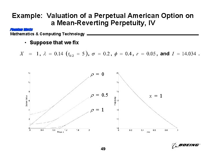
Example: Valuation of a Perpetual American Option on a Mean-Reverting Perpetuity, IV Phantom Works Mathematics & Computing Technology • Suppose that we fix = 0. 5 = 1 49 x = 1

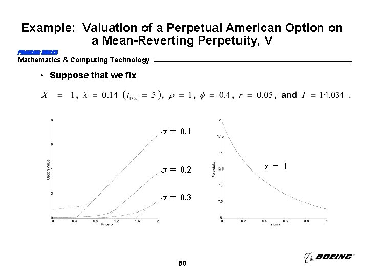
Example: Valuation of a Perpetual American Option on a Mean-Reverting Perpetuity, V Phantom Works Mathematics & Computing Technology • Suppose that we fix = 0. 1 = 0. 2 = 0. 3 50 x = 1

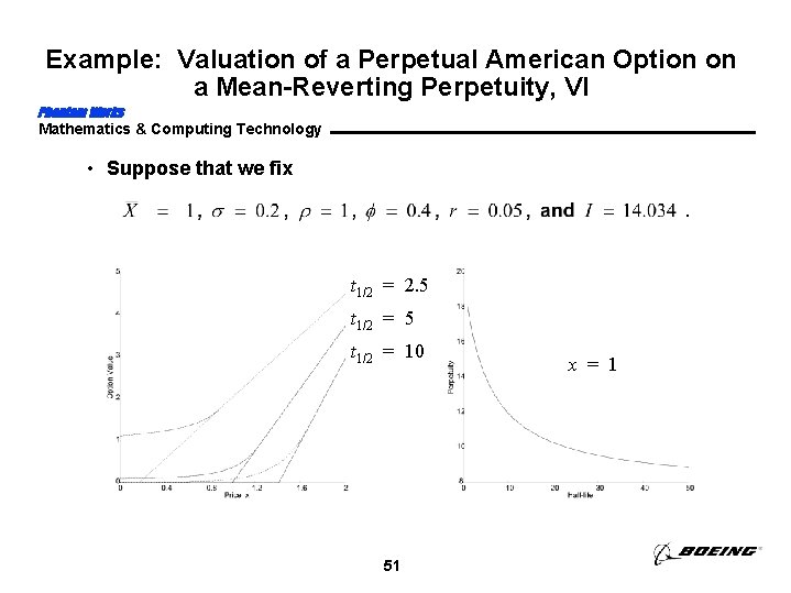
Example: Valuation of a Perpetual American Option on a Mean-Reverting Perpetuity, VI Phantom Works Mathematics & Computing Technology • Suppose that we fix t 1/2 = 2. 5 t 1/2 = 10 51 x = 1

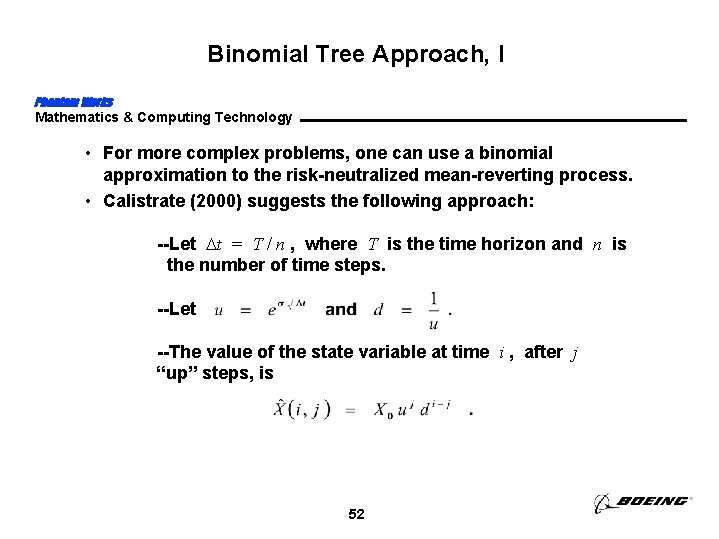
Binomial Tree Approach, I Phantom Works Mathematics & Computing Technology • For more complex problems, one can use a binomial approximation to the risk-neutralized mean-reverting process. • Calistrate (2000) suggests the following approach: --Let t = T / n , where T is the time horizon and n is the number of time steps. --Let --The value of the state variable at time i , after j “up” steps, is 52

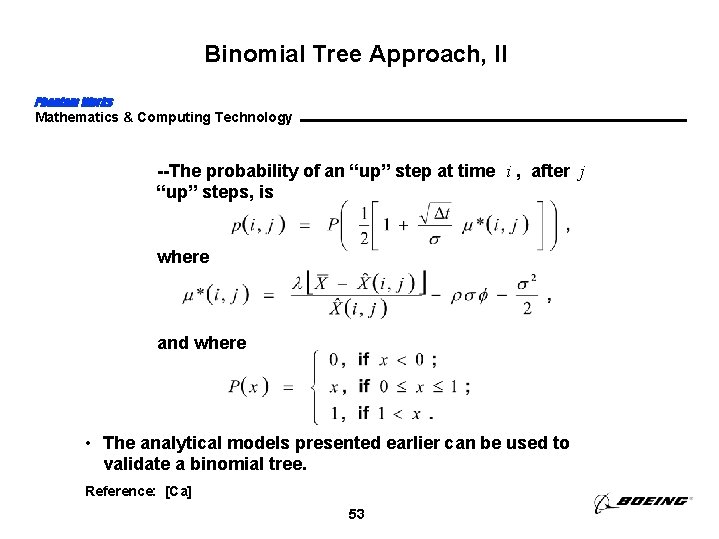
Binomial Tree Approach, II Phantom Works Mathematics & Computing Technology --The probability of an “up” step at time i , after j “up” steps, is where and where • The analytical models presented earlier can be used to validate a binomial tree. Reference: [Ca] 53

Conclusion Phantom Works Mathematics & Computing Technology • Of the models we have considered for a mean-reverting price process, inhomogeneous geometric Brownian motion is the most appropriate. --It is guaranteed to be positive --One can compute its moments --It really does revert to a mean --It has an appealing homogeneity property --The available evidence suggests that it is (at least approximately) lognormal • Bhattacharya (1978) showed how to value certain cash flow streams which depend on such a process. • We have shown how to value certain options on such cash flow streams. 54

References, I Phantom Works Mathematics & Computing Technology [B] [BØ] [Ca] [Co. A] [DP] S. Bhattacharya, “Project Valuation with Mean-Reverting Cash Flow Streams, ” Journal of Finance 33, December 1978, pp. 1317 -1331. K. Brekke and B. Øksendal, “The High Contact Principle as a Sufficiency Condition for Optimal Stopping. ” Stochastic Models and Option Values, D. Lund and B. Øksendal, editors, Elsevier Science Publishers, 1991, pp. 187 -208. D. Calistrate, “Setting Lattice Parameters for Derivatives Valuation”, private communication, 2000. G. Constantinides, “Market Risk Adjustment in Project Valuation, ” Journal of Finance 33, May 1978, pp. 603 -616. T. Copeland V. Antikarov, Real Options: A Practitioner’s Guide, Texere, 2001. A. Dixit and R. Pindyck, Investment under Uncertainty, Princeton University Press, 1994. 55

References, II Phantom Works Mathematics & Computing Technology [KP] P. Kloeden and E. Platen, Numerical Solution of Stochastic Differential Equations, Springer-Verlag, 1992. [L] Y. Luke, “Algorithms for Rational Approximations for a Confluent Hypergeometric Function, ” Utilitas Math. 11 (1977), pp. 123 -151. [Mc. DS] R. Mc. Donald and D. Siegel, “The Value of Waiting to Invest, ” Quarterly J. Econ. 101 (1986), pp. 707 -728. [Pil] D. Pilipovic, Energy Risk, Mc. Graw-Hill, 1998. [Pin] R. Pindyck, “Irreversibility, Uncertainty, and Investment, ” J. Econ. Lit. 19 (1991), pp. 1110 -1148. [R] B. L. S. Prakasa Rao, Statistical Inference for Diffusion Type Processes (Kendall’s Library of Statistics 8), Arnold / Oxford University Press, 1999. [Sh] D. Shimko, Finance in Continuous Time--A Primer, Kolb, 1992. 56

References, III Phantom Works Mathematics & Computing Technology [Si] [SO] [Sp. O] [T] [W] G. Sick, “Real Options. ” Finance (Handbooks in Operations Research and Management Science, Volume 9), R. Jarrow, V. Maksimovic, and W. Ziemba, editors, pp. 631 -691, North-Holland, 1995. I. Shoji and T. Ozaki, “Comparative Study of Estimation Methods for Continuous Time Stochastic Processes, ” J. Time Series Analysis 18 (1997), pp. 485 -506. J. Spanier and K. Oldham, An Atlas of Functions, Hemisphere, 1987. L. Trigeorgis, Real Options, MIT Press, 1996. P. Wilmott, Paul Wilmott on Quantitative Finance, Wiley, 2000. 57