Personal Genomics Phasing and imputation Shai Carmi School

Personal Genomics Phasing and imputation Shai Carmi School of Public Health

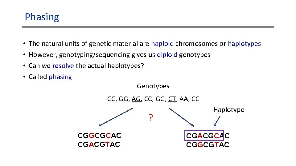
Phasing • • The natural units of genetic material are haploid chromosomes or haplotypes However, genotyping/sequencing gives us diploid genotypes Can we resolve the actual haplotypes? Called phasing Genotypes CC, GG, AG, CC, GG, CT, AA, CC ? CGGCGCAC CGACGTAC Haplotype CGACGCAC CGGCGTAC

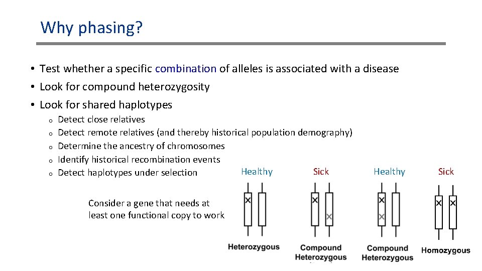
Why phasing? • Test whether a specific combination of alleles is associated with a disease • Look for compound heterozygosity • Look for shared haplotypes o o o Detect close relatives Detect remote relatives (and thereby historical population demography) Determine the ancestry of chromosomes Identify historical recombination events Healthy Sick Detect haplotypes under selection Consider a gene that needs at least one functional copy to work Healthy Sick

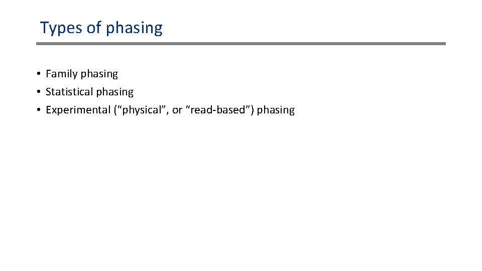
Types of phasing • Family phasing • Statistical phasing • Experimental (“physical”, or “read-based”) phasing

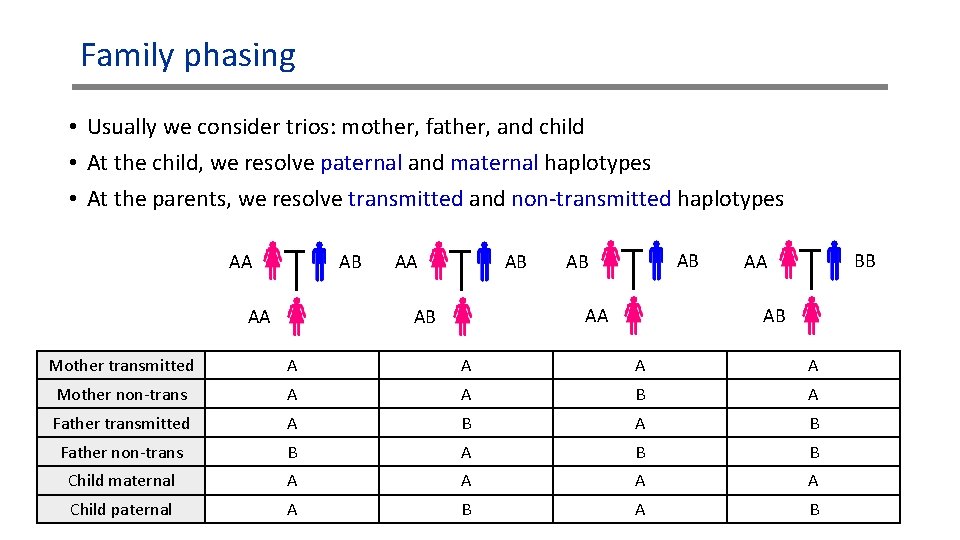
Family phasing • Usually we consider trios: mother, father, and child • At the child, we resolve paternal and maternal haplotypes • At the parents, we resolve transmitted and non-transmitted haplotypes AB AA AA AB AB AA AB BB AA AB Mother transmitted A A Mother non-trans A A B A Father transmitted A B Father non-trans B A B B Child maternal A A Child paternal A B

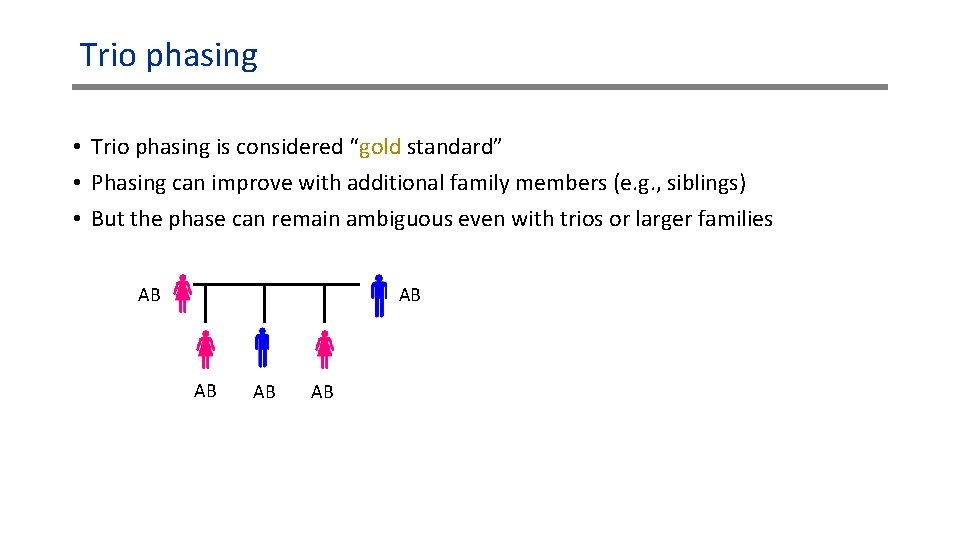
Trio phasing • Trio phasing is considered “gold standard” • Phasing can improve with additional family members (e. g. , siblings) • But the phase can remain ambiguous even with trios or larger families AB AB AB

Statistical phasing • For each single target genome, no information is available to allow phasing • But we can look for other individuals who are homozygous to the same haplotypes! • Homozygous individuals have two copies of the same haplotype, so no ambiguity • Even when there is one het, there is no ambiguity • The presence of a haplotype in one individual does not guarantee that the same haplotype will be found in another • But it is quite likely, due to linkage disequilibrium (correlation along the genome) o More later

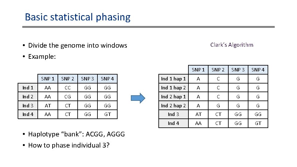
Basic statistical phasing • Divide the genome into windows • Example: Clark’s Algorithm SNP 1 SNP 2 SNP 3 SNP 4 Ind 1 hap 1 A C G G Ind 1 AA CC GG GG Ind 1 hap 2 A C G G Ind 2 AA CG GG GG Ind 2 hap 1 A C G G Ind 3 AT CT GG GG Ind 2 hap 2 A G G G Ind 4 AA CT GG GT Ind 3 AT CT GG GG Ind 4 AA CT GG GT • Haplotype “bank”: ACGG, AGGG • How to phase individual 3?

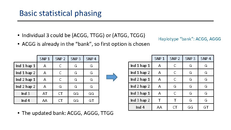
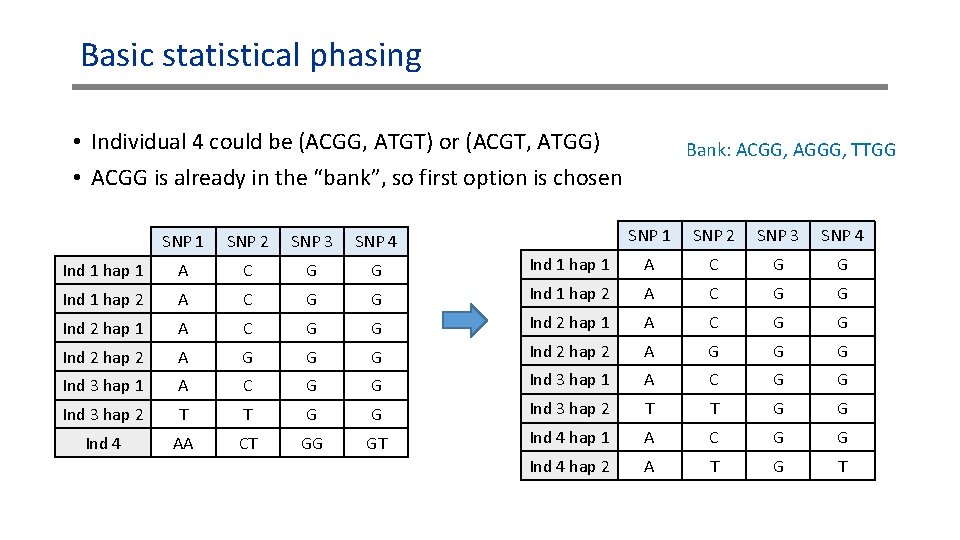
Basic statistical phasing • Individual 3 could be (ACGG, TTGG) or (ATGG, TCGG) • ACGG is already in the “bank”, so first option is chosen Haplotype “bank”: ACGG, AGGG SNP 1 SNP 2 SNP 3 SNP 4 Ind 1 hap 1 A C G G G Ind 1 hap 2 A C G G Ind 2 hap 1 A C G G G Ind 2 hap 2 A G G G AT CT GG GG Ind 3 hap 1 A C G G AA CT GG GT Ind 3 hap 2 T T G G Ind 4 AA CT GG GT SNP 1 SNP 2 SNP 3 SNP 4 Ind 1 hap 1 A C G G Ind 1 hap 2 A C G Ind 2 hap 1 A C Ind 2 hap 2 A Ind 3 Ind 4 • The updated bank: ACGG, AGGG, TTGG

Basic statistical phasing • Individual 4 could be (ACGG, ATGT) or (ACGT, ATGG) • ACGG is already in the “bank”, so first option is chosen Bank: ACGG, AGGG, TTGG SNP 1 SNP 2 SNP 3 SNP 4 Ind 1 hap 1 A C G G G Ind 1 hap 2 A C G G Ind 2 hap 1 A C G G G Ind 2 hap 2 A G G G A C G G Ind 3 hap 1 A C G G Ind 3 hap 2 T T G G Ind 4 AA CT GG GT Ind 4 hap 1 A C G G Ind 4 hap 2 A T G T SNP 1 SNP 2 SNP 3 SNP 4 Ind 1 hap 1 A C G G Ind 1 hap 2 A C G Ind 2 hap 1 A C Ind 2 hap 2 A Ind 3 hap 1

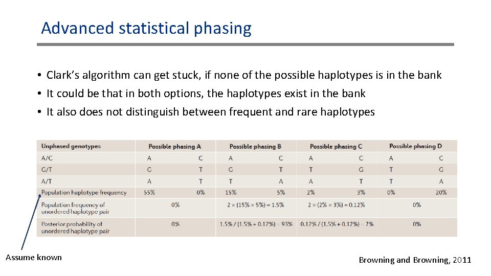
Advanced statistical phasing • Clark’s algorithm can get stuck, if none of the possible haplotypes is in the bank • It could be that in both options, the haplotypes exist in the bank • It also does not distinguish between frequent and rare haplotypes Assume known Browning and Browning, 2011

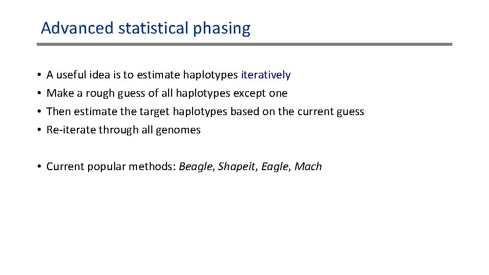
Advanced statistical phasing • • A useful idea is to estimate haplotypes iteratively Make a rough guess of all haplotypes except one Then estimate the target haplotypes based on the current guess Re-iterate through all genomes • Current popular methods: Beagle, Shapeit, Eagle, Mach

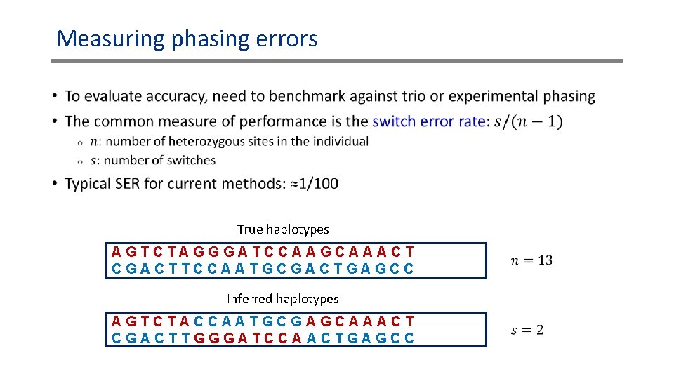
Measuring phasing errors • True haplotypes AGTCTAGGGATCCAAGCAAACT CGACTTCCAATGCGACTGAGCC Inferred haplotypes AGTCTACCAATGCGAGCAAACT CGACTTGGGATCCAACTGAGCC

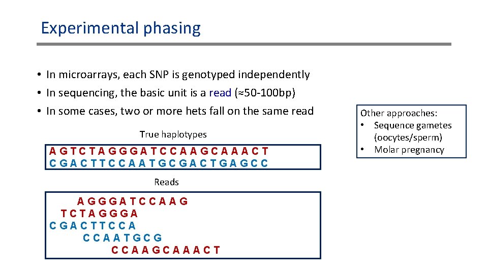
Experimental phasing • In microarrays, each SNP is genotyped independently • In sequencing, the basic unit is a read (≈50 -100 bp) • In some cases, two or more hets fall on the same read True haplotypes AGTCTAGGGATCCAAGCAAACT CGACTTCCAATGCGACTGAGCC Reads AGGGATCCAAG TCTAGGGA CGACTTCCA CCAATGCG CCAAGCAAACT Other approaches: • Sequence gametes (oocytes/sperm) • Molar pregnancy

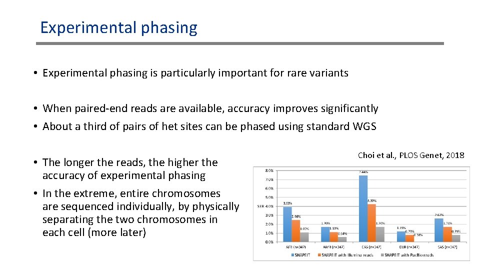
Experimental phasing • Experimental phasing is particularly important for rare variants • When paired-end reads are available, accuracy improves significantly • About a third of pairs of het sites can be phased using standard WGS • The longer the reads, the higher the accuracy of experimental phasing • In the extreme, entire chromosomes are sequenced individually, by physically separating the two chromosomes in each cell (more later) Choi et al. , PLOS Genet, 2018

What about the missing variants? • Microarrays are ≈20 x cheaper than WGS, but only cover ≈1 M sites out of ≈3 B • While the selection is educated (polymorphic/important sites), many variants remain uncovered • Fortunately, this is in many cases good enough! • The genotyped SNPs are linked to ungenotyped SNPs • Linkage = correlation • Also called linkage disequilibrium (LD)

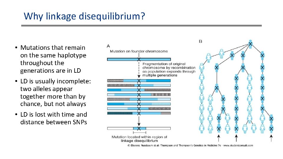
Why linkage disequilibrium? • Mutations that remain on the same haplotype throughout the generations are in LD • LD is usually incomplete: two alleles appear together more than by chance, but not always • LD is lost with time and distance between SNPs

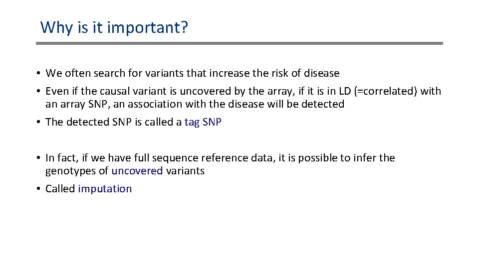
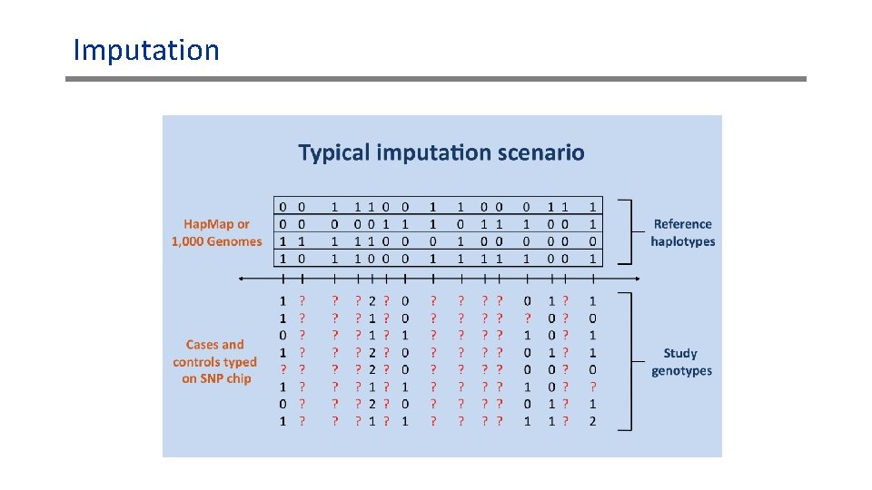
Why is it important? • We often search for variants that increase the risk of disease • Even if the causal variant is uncovered by the array, if it is in LD (=correlated) with an array SNP, an association with the disease will be detected • The detected SNP is called a tag SNP • In fact, if we have full sequence reference data, it is possible to infer the genotypes of uncovered variants • Called imputation

Imputation

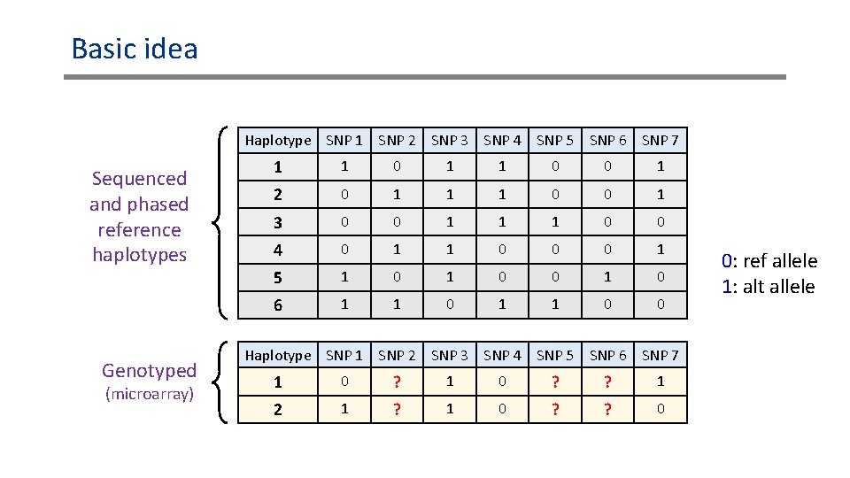
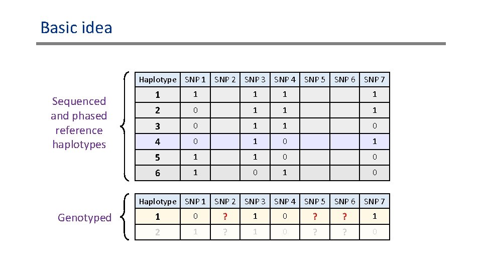
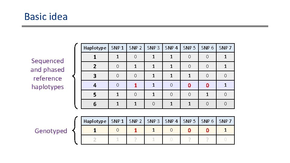
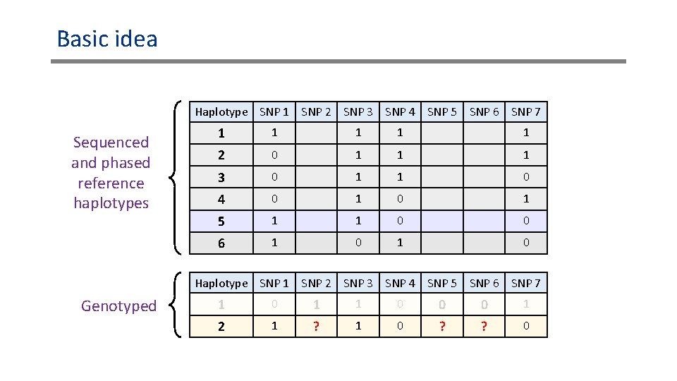
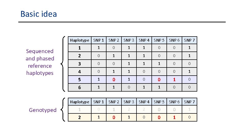
Basic idea • Divide the genome into windows • Collect a set of previously phased fully sequenced reference haplotypes • For each window, detect the reference haplotype most similar to the target genome, only based on the array SNPs • Infer the genotypes at ungenotyped SNPs according to the reference sequence

Basic idea Haplotype SNP 1 SNP 2 SNP 3 SNP 4 SNP 5 SNP 6 SNP 7 Sequenced and phased reference haplotypes Genotyped (microarray) 1 1 0 0 1 2 0 1 1 1 0 0 1 3 0 0 1 1 1 0 0 4 0 1 1 0 0 0 1 5 1 0 0 1 0 6 1 1 0 0 Haplotype SNP 1 SNP 2 SNP 3 SNP 4 SNP 5 SNP 6 SNP 7 1 0 ? ? 1 2 1 ? 1 0 ? ? 0 0: ref allele 1: alt allele

Basic idea Haplotype SNP 1 SNP 2 SNP 3 SNP 4 SNP 5 SNP 6 SNP 7 Sequenced and phased reference haplotypes 1 1 1 2 0 1 1 1 3 0 1 1 0 4 0 1 5 1 1 0 0 6 1 0 Haplotype SNP 1 SNP 2 SNP 3 SNP 4 SNP 5 SNP 6 SNP 7 Genotyped 1 0 ? ? 1 2 1 ? 1 0 ? ? 0

Basic idea Haplotype SNP 1 SNP 2 SNP 3 SNP 4 SNP 5 SNP 6 SNP 7 Sequenced and phased reference haplotypes 1 1 0 0 1 2 0 1 1 1 0 0 1 3 0 0 1 1 1 0 0 4 0 1 1 0 0 0 1 5 1 0 0 1 0 6 1 1 0 0 Haplotype SNP 1 SNP 2 SNP 3 SNP 4 SNP 5 SNP 6 SNP 7 Genotyped 1 0 1 1 0 0 0 1 2 1 ? 1 0 ? ? 0

Basic idea Haplotype SNP 1 SNP 2 SNP 3 SNP 4 SNP 5 SNP 6 SNP 7 Sequenced and phased reference haplotypes 1 1 1 2 0 1 1 1 3 0 1 1 0 4 0 1 5 1 1 0 0 6 1 0 Haplotype SNP 1 SNP 2 SNP 3 SNP 4 SNP 5 SNP 6 SNP 7 Genotyped 1 0 1 1 0 0 0 1 2 1 ? 1 0 ? ? 0

Basic idea Haplotype SNP 1 SNP 2 SNP 3 SNP 4 SNP 5 SNP 6 SNP 7 Sequenced and phased reference haplotypes 1 1 0 0 1 2 0 1 1 1 0 0 1 3 0 0 1 1 1 0 0 4 0 1 1 0 0 0 1 5 1 0 0 1 0 6 1 1 0 0 Haplotype SNP 1 SNP 2 SNP 3 SNP 4 SNP 5 SNP 6 SNP 7 Genotyped 1 0 1 2 2 0 0 1 2 1 0 0 1 0

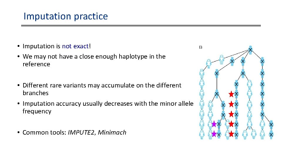
Imputation practice • Imputation is not exact! • We may not have a close enough haplotype in the reference • Different rare variants may accumulate on the different branches • Imputation accuracy usually decreases with the minor allele frequency • Common tools: IMPUTE 2, Minimach

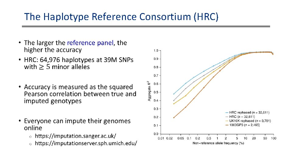
The Haplotype Reference Consortium (HRC) •

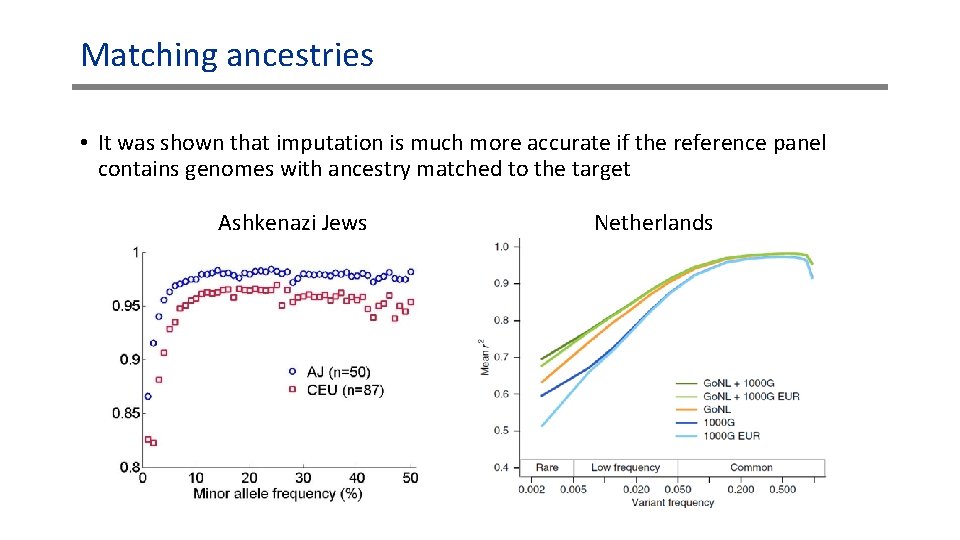
Matching ancestries • It was shown that imputation is much more accurate if the reference panel contains genomes with ancestry matched to the target Ashkenazi Jews Netherlands

What’s still missing? • All the algorithms we have so far described work by dividing the genome into windows • But. . . • How to choose the window size and boundaries? • How to avoid discontinuities between windows? • It is better to avoid windows altogether, using Hidden Markov Models (HMM)

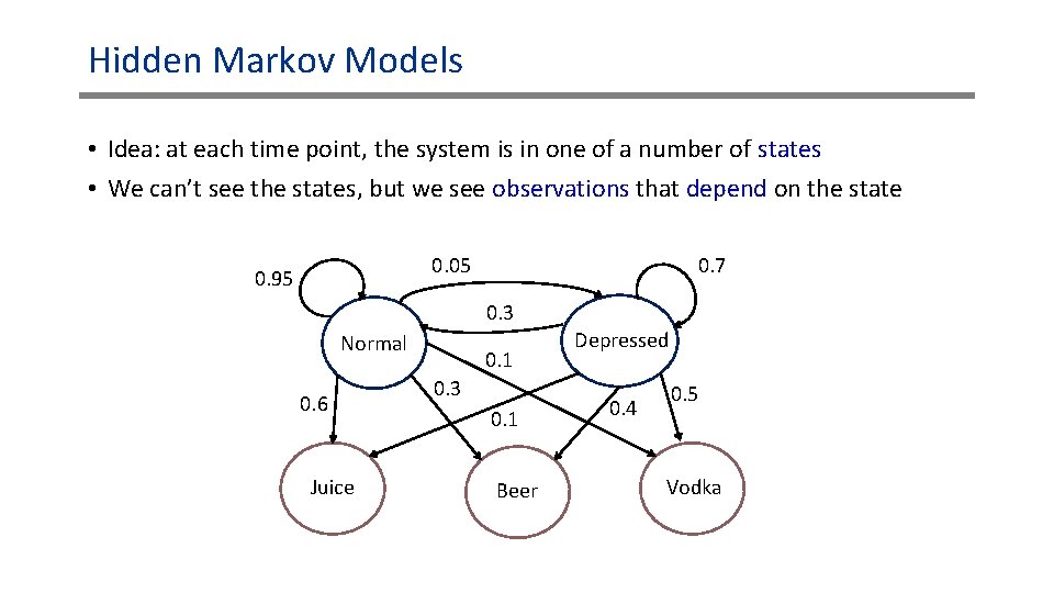
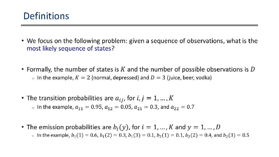
Hidden Markov Models • Idea: at each time point, the system is in one of a number of states • We can’t see the states, but we see observations that depend on the state 0. 7 0. 05 0. 95 0. 3 Normal 0. 6 Juice 0. 1 0. 3 0. 1 Beer Depressed 0. 4 0. 5 Vodka

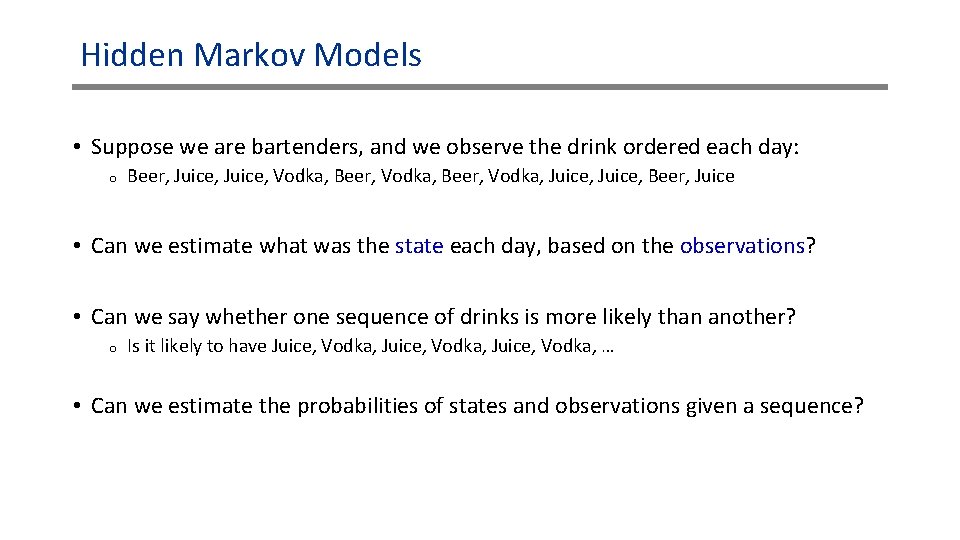
Hidden Markov Models • Suppose we are bartenders, and we observe the drink ordered each day: o Beer, Juice, Vodka, Beer, Vodka, Juice, Beer, Juice • Can we estimate what was the state each day, based on the observations? • Can we say whether one sequence of drinks is more likely than another? o Is it likely to have Juice, Vodka, … • Can we estimate the probabilities of states and observations given a sequence?

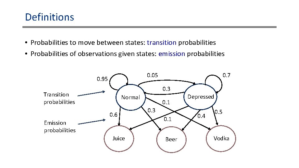
Definitions • Probabilities to move between states: transition probabilities • Probabilities of observations given states: emission probabilities 0. 7 0. 05 0. 95 0. 3 Transition probabilities Normal 0. 6 Emission probabilities Juice 0. 1 0. 3 0. 1 Beer Depressed 0. 4 0. 5 Vodka

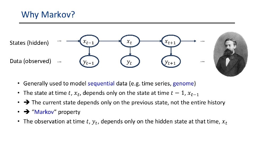
Why Markov? … … Data (observed) … … States (hidden) •

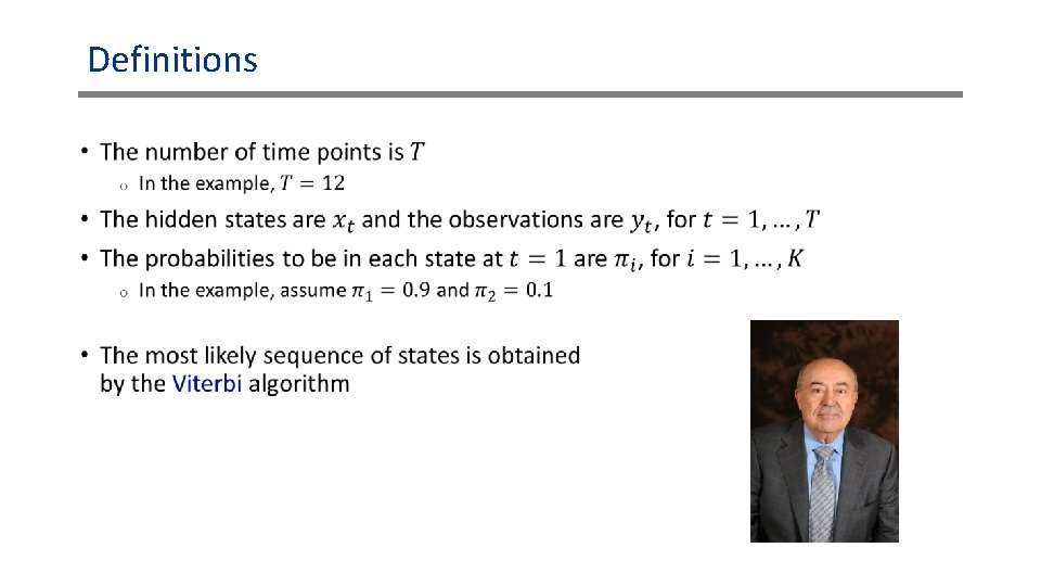
Definitions •

Definitions •

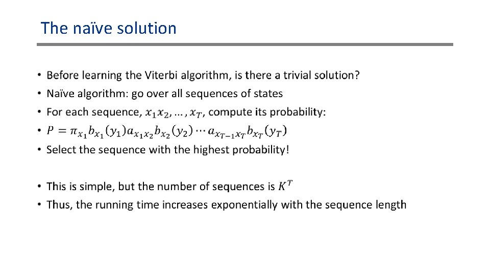
The naïve solution •

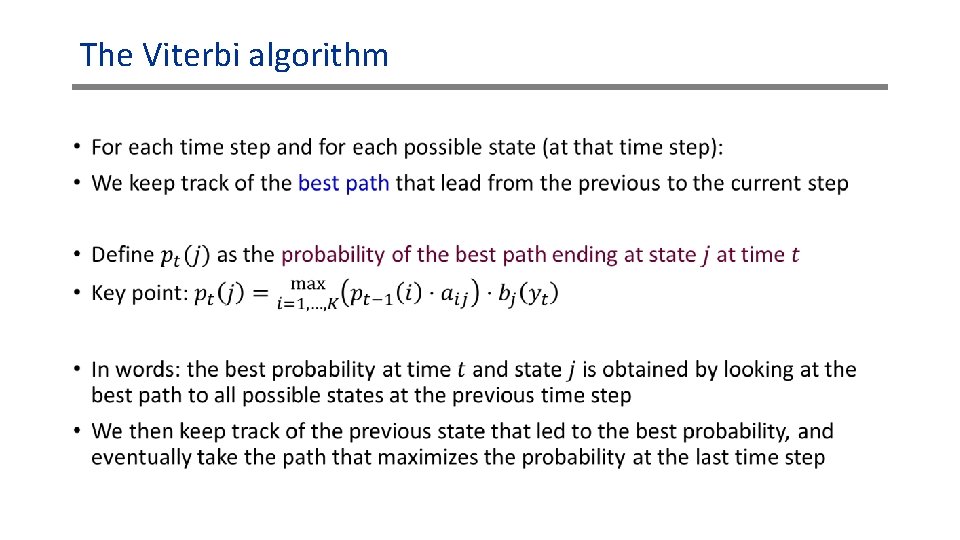
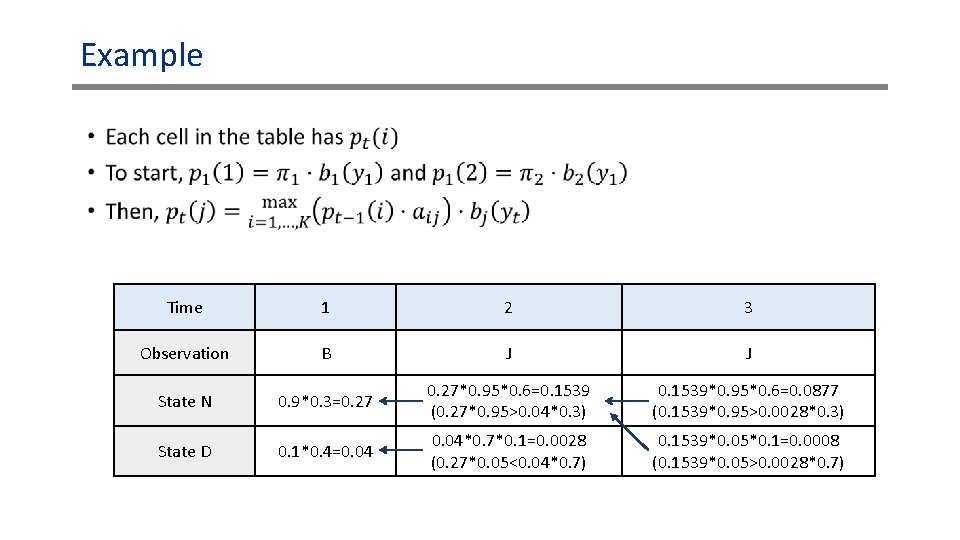
The Viterbi algorithm •

Example • Time 1 2 3 Observation B J J State N 0. 9*0. 3=0. 27*0. 95*0. 6=0. 1539 (0. 27*0. 95>0. 04*0. 3) 0. 1539*0. 95*0. 6=0. 0877 (0. 1539*0. 95>0. 0028*0. 3) State D 0. 1*0. 4=0. 04*0. 7*0. 1=0. 0028 (0. 27*0. 05<0. 04*0. 7) 0. 1539*0. 05*0. 1=0. 0008 (0. 1539*0. 05>0. 0028*0. 7)

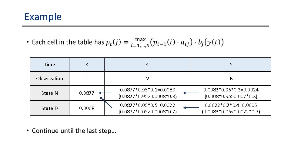
Example • Time 3 4 5 Observation J V B State N 0. 0877*0. 95*0. 1=0. 0083 (0. 0877*0. 95>0. 0008*0. 3) 0. 0083*0. 95*0. 3=0. 0024 (0. 008*0. 95>0. 002*0. 3) State D 0. 0008 0. 0877*0. 05*0. 5=0. 0022 (0. 0877*0. 05>0. 0008*0. 7) 0. 0022*0. 7*0. 4=0. 0006 (0. 0083*0. 05<0. 0022*0. 7)

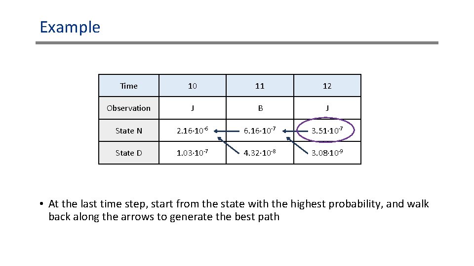
Example Time 10 11 12 Observation J B J State N 2. 16∙ 10 -6 6. 16∙ 10 -7 3. 51∙ 10 -7 State D 1. 03∙ 10 -7 4. 32∙ 10 -8 3. 08∙ 10 -9 • At the last time step, start from the state with the highest probability, and walk back along the arrows to generate the best path

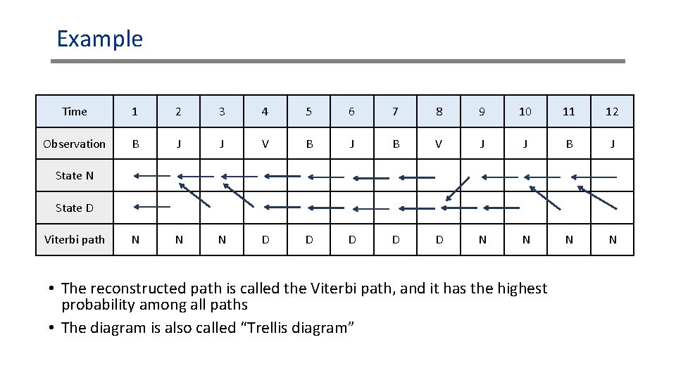
Example Time 1 2 3 4 5 6 7 8 9 10 11 12 Observation B J J V B J B V J J B J N N N D D D N N State D Viterbi path • The reconstructed path is called the Viterbi path, and it has the highest probability among all paths • The diagram is also called “Trellis diagram”

Remarks •

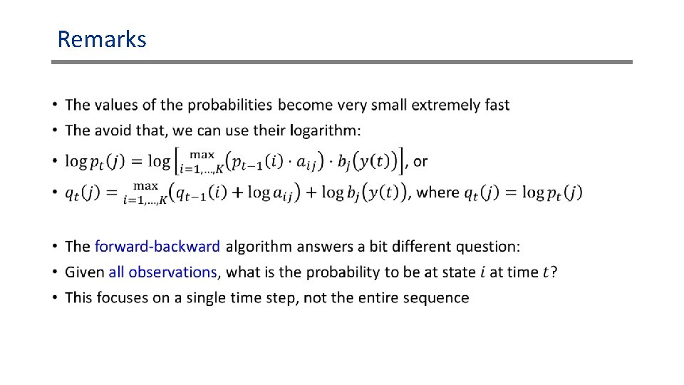
Remarks •

How is it related to imputation? •

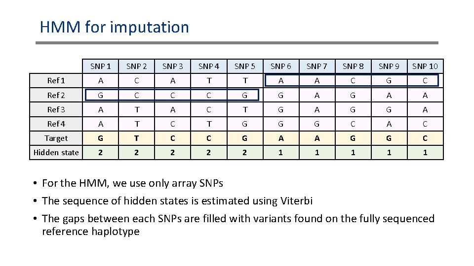
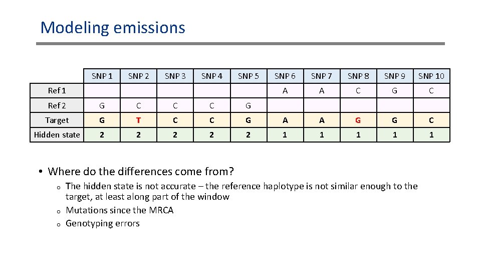
HMM for imputation SNP 1 SNP 2 SNP 3 SNP 4 SNP 5 SNP 6 SNP 7 SNP 8 SNP 9 SNP 10 Ref 1 A C A T T A A C G C Ref 2 G C C C G G A A Ref 3 A T A C T G A G G A Ref 4 A T C T G G G C A C Target G T C C G A A G G C Hidden state 2 2 2 1 1 1 • For the HMM, we use only array SNPs • The sequence of hidden states is estimated using Viterbi • The gaps between each SNPs are filled with variants found on the fully sequenced reference haplotype

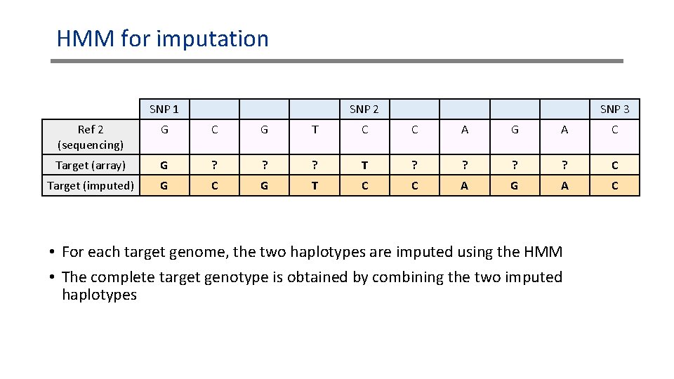
HMM for imputation SNP 1 SNP 2 SNP 3 Ref 2 (sequencing) G C G T C C A G A C Target (array) G ? ? ? T ? ? C Target (imputed) G C G T C C A G A C • For each target genome, the two haplotypes are imputed using the HMM • The complete target genotype is obtained by combining the two imputed haplotypes

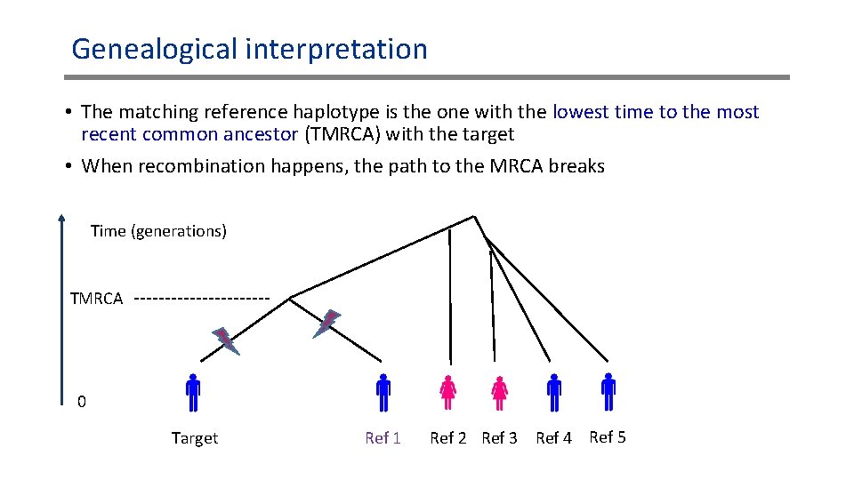
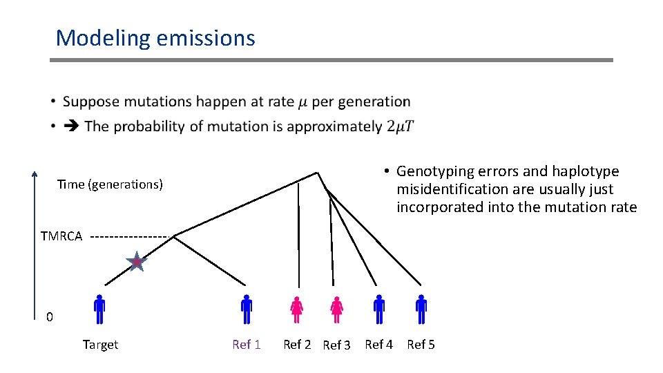
Genealogical interpretation • The matching reference haplotype is the one with the lowest time to the most recent common ancestor (TMRCA) with the target • When recombination happens, the path to the MRCA breaks Time (generations) TMRCA 0 Target Ref 1 Ref 2 Ref 3 Ref 4 Ref 5

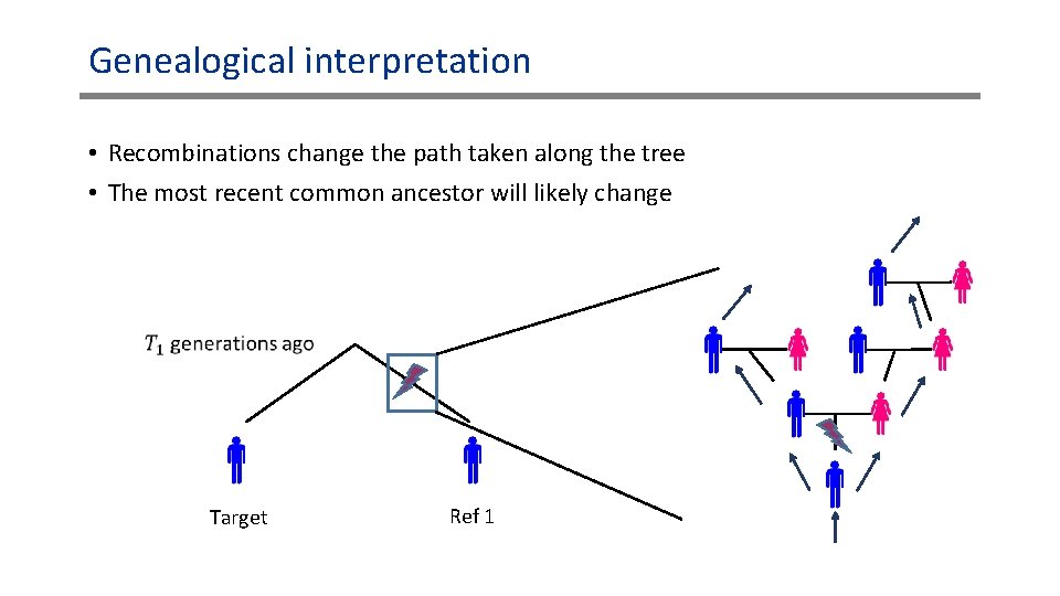
Genealogical interpretation • Recombinations change the path taken along the tree • The most recent common ancestor will likely change Target Ref 1

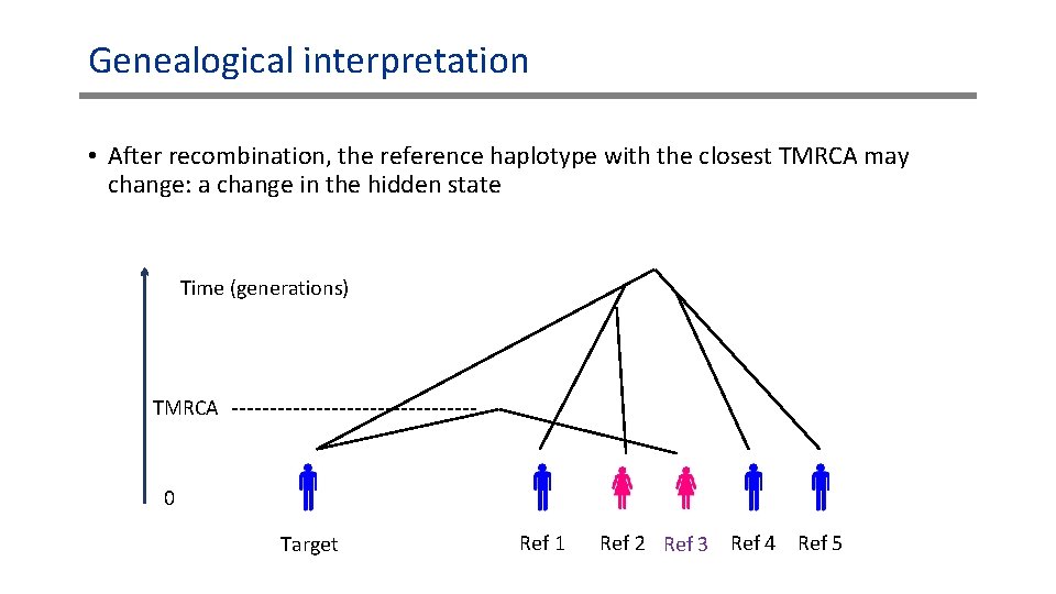
Genealogical interpretation • After recombination, the reference haplotype with the closest TMRCA may change: a change in the hidden state Time (generations) TMRCA 0 Target Ref 1 Ref 2 Ref 3 Ref 4 Ref 5

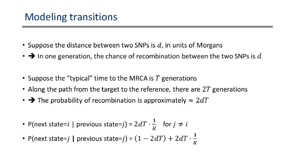
Modeling transitions •

Modeling emissions SNP 1 SNP 2 SNP 3 SNP 4 SNP 5 Ref 1 SNP 6 SNP 7 SNP 8 SNP 9 SNP 10 A A C G C Ref 2 G C C C G Target G T C C G A A G G C Hidden state 2 2 2 1 1 1 • Where do the differences come from? o o o The hidden state is not accurate – the reference haplotype is not similar enough to the target, at least along part of the window Mutations since the MRCA Genotyping errors

Modeling emissions • • Genotyping errors and haplotype misidentification are usually just incorporated into the mutation rate Time (generations) TMRCA 0 Target Ref 1 Ref 2 Ref 3 Ref 4 Ref 5

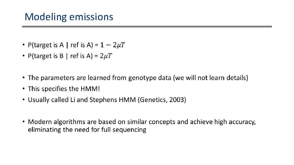
Modeling emissions •