Perceptron as one Type of Linear Discriminants 1

Perceptron as one Type of Linear Discriminants 1 • Introduction • Design of Primitive Units • • Perceptrons Security applications of perceptron

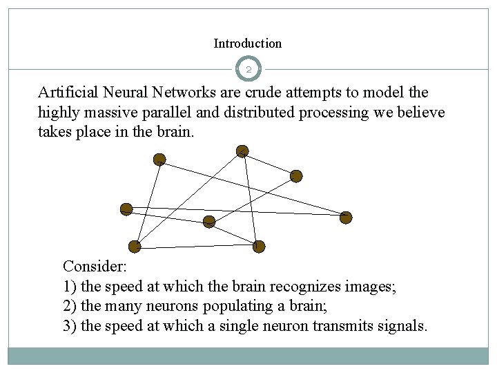
Introduction 2 Artificial Neural Networks are crude attempts to model the highly massive parallel and distributed processing we believe takes place in the brain. Consider: 1) the speed at which the brain recognizes images; 2) the many neurons populating a brain; 3) the speed at which a single neuron transmits signals.

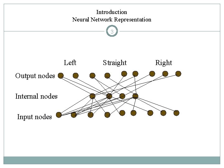
Introduction Neural Network Representation 3 Left Output nodes Internal nodes Input nodes Straight Right

Introduction Problems for Neural Networks 4 ü Examples may be described by a large number of attributes (e. g. , pixels in an image). ü The output value can be discrete, continuous, or a vector of either discrete or continuous values. ü Data may contain errors. ü The time for training may be extremely long. ü Evaluating the network for a new example is relatively fast. ü Interpretability of the final hypothesis is not relevant (the NN is treated as a black box).

Perceptron as one Type of Linear Discriminants 5 • Introduction • Design of Primitive Units • Perceptrons

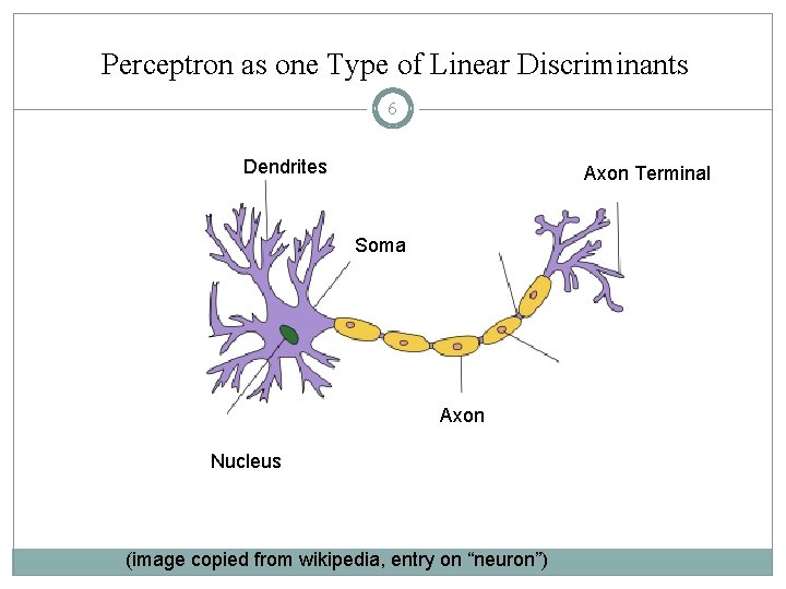
Perceptron as one Type of Linear Discriminants 6 Dendrites Axon Terminal Soma Axon Nucleus (image copied from wikipedia, entry on “neuron”)

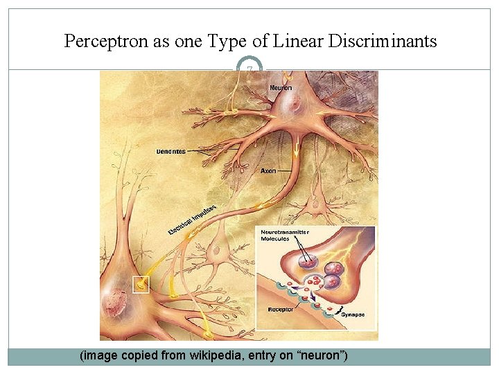
Perceptron as one Type of Linear Discriminants 7 (image copied from wikipedia, entry on “neuron”)

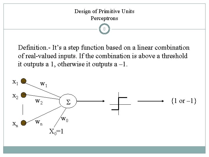
Design of Primitive Units Perceptrons 8 Definition. - It’s a step function based on a linear combination of real-valued inputs. If the combination is above a threshold it outputs a 1, otherwise it outputs a – 1. x 1 x 2 xn w 1 w 2 wn Σ w 0 X 0=1 {1 or – 1}

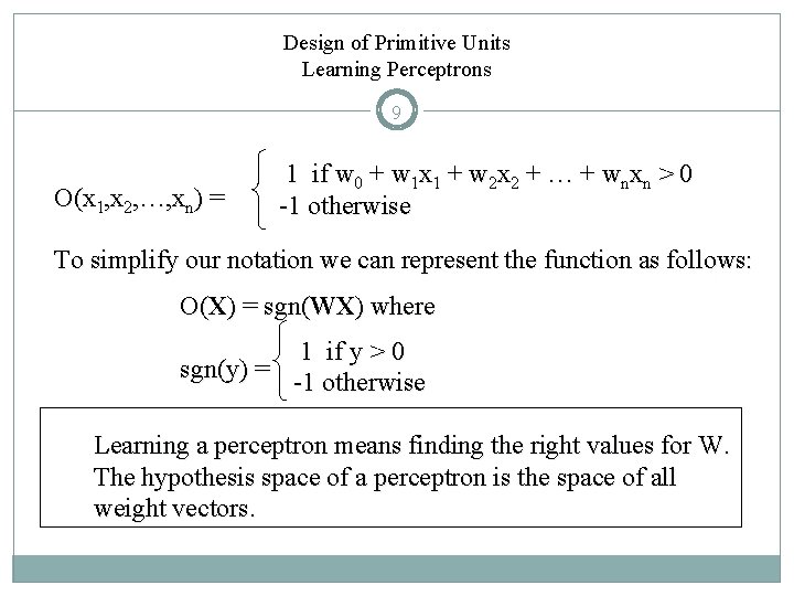
Design of Primitive Units Learning Perceptrons 9 O(x 1, x 2, …, xn) = 1 if w 0 + w 1 x 1 + w 2 x 2 + … + wnxn > 0 -1 otherwise To simplify our notation we can represent the function as follows: O(X) = sgn(WX) where 1 if y > 0 sgn(y) = -1 otherwise Learning a perceptron means finding the right values for W. The hypothesis space of a perceptron is the space of all weight vectors.

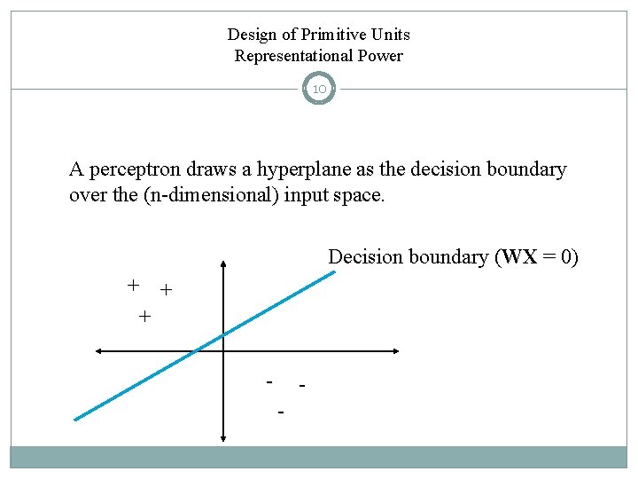
Design of Primitive Units Representational Power 10 A perceptron draws a hyperplane as the decision boundary over the (n-dimensional) input space. Decision boundary (WX = 0) + + + - -

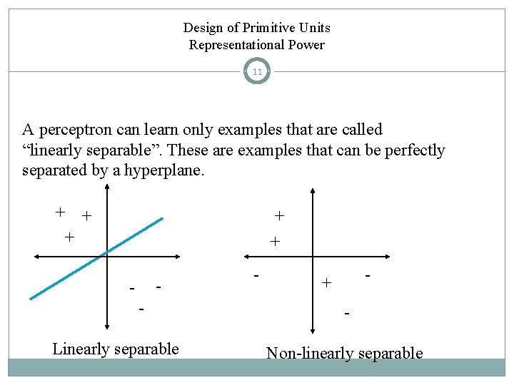
Design of Primitive Units Representational Power 11 A perceptron can learn only examples that are called “linearly separable”. These are examples that can be perfectly separated by a hyperplane. + + + - - Linearly separable - - + - Non-linearly separable

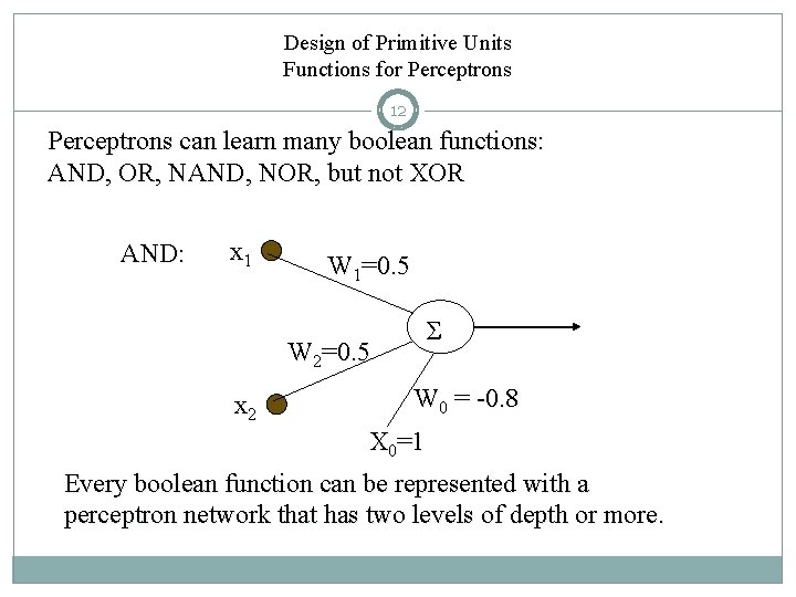
Design of Primitive Units Functions for Perceptrons 12 Perceptrons can learn many boolean functions: AND, OR, NAND, NOR, but not XOR AND: x 1 W 1=0. 5 Σ W 2=0. 5 x 2 W 0 = -0. 8 X 0=1 Every boolean function can be represented with a perceptron network that has two levels of depth or more.

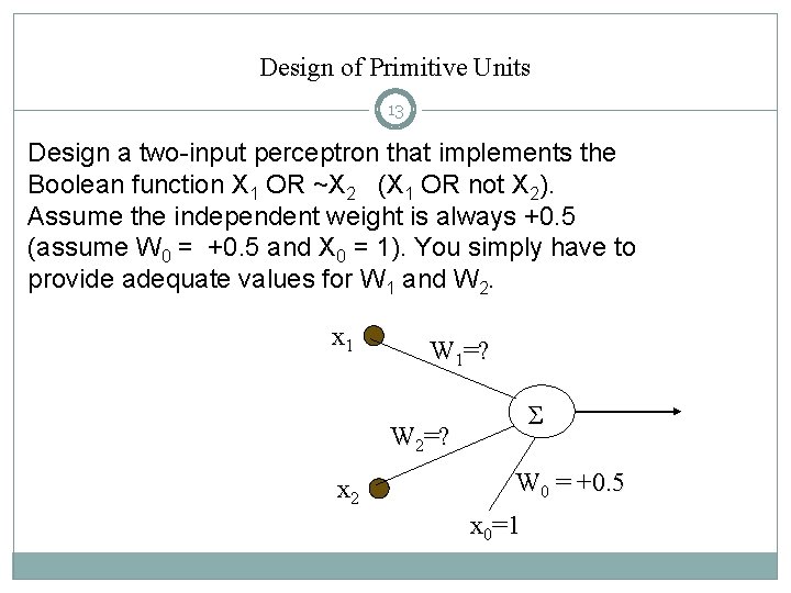
Design of Primitive Units 13 Design a two-input perceptron that implements the Boolean function X 1 OR ~X 2 (X 1 OR not X 2). Assume the independent weight is always +0. 5 (assume W 0 = +0. 5 and X 0 = 1). You simply have to provide adequate values for W 1 and W 2. x 1 W 1=? Σ W 2=? x 2 W 0 = +0. 5 x 0=1

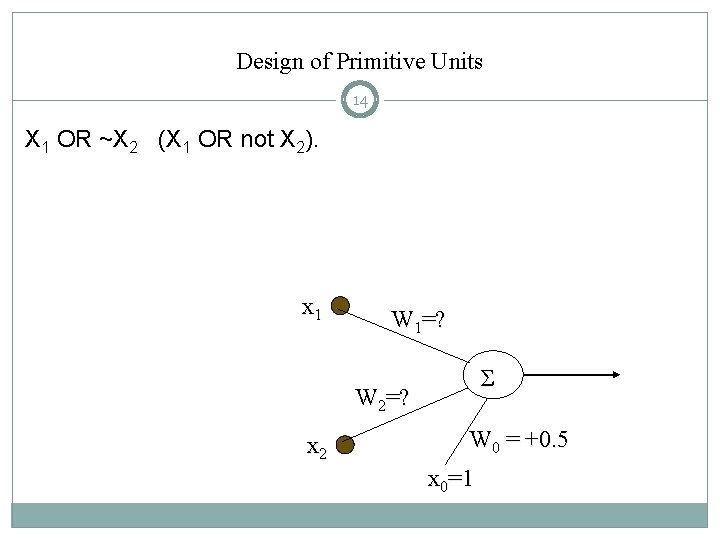
Design of Primitive Units 14 X 1 OR ~X 2 (X 1 OR not X 2). x 1 W 1=? Σ W 2=? x 2 W 0 = +0. 5 x 0=1

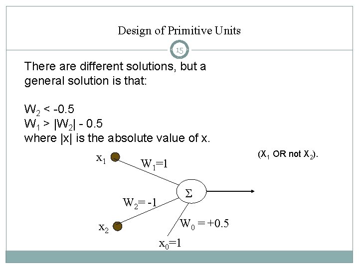
Design of Primitive Units 15 There are different solutions, but a general solution is that: W 2 < -0. 5 W 1 > |W 2| - 0. 5 where |x| is the absolute value of x. x 1 (X 1 OR not X 2). W 1=1 Σ W 2= -1 x 2 W 0 = +0. 5 x 0=1

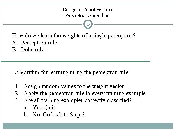
Design of Primitive Units Perceptron Algorithms 16 How do we learn the weights of a single perceptron? A. Perceptron rule B. Delta rule Algorithm for learning using the perceptron rule: 1. Assign random values to the weight vector 2. Apply the perceptron rule to every training example 3. Are all training examples correctly classified? a. Yes. Quit b. No. Go back to Step 2.

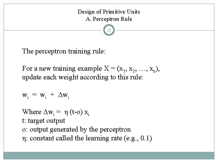
Design of Primitive Units A. Perceptron Rule 17 The perceptron training rule: For a new training example X = (x 1, x 2, …, xn), update each weight according to this rule: wi = wi + Δwi Where Δwi = η (t-o) xi t: target output o: output generated by the perceptron η: constant called the learning rate (e. g. , 0. 1)

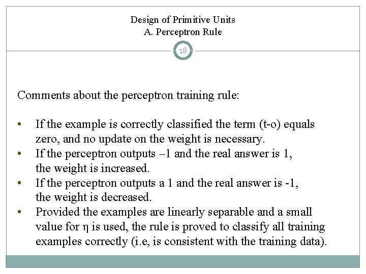
Design of Primitive Units A. Perceptron Rule 18 Comments about the perceptron training rule: • • If the example is correctly classified the term (t-o) equals zero, and no update on the weight is necessary. If the perceptron outputs – 1 and the real answer is 1, the weight is increased. If the perceptron outputs a 1 and the real answer is -1, the weight is decreased. Provided the examples are linearly separable and a small value for η is used, the rule is proved to classify all training examples correctly (i. e, is consistent with the training data).

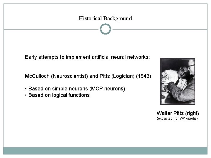
Historical Background Early attempts to implement artificial neural networks: Mc. Culloch (Neuroscientist) and Pitts (Logician) (1943) • Based on simple neurons (MCP neurons) • Based on logical functions Walter Pitts (right) (extracted from Wikipedia)

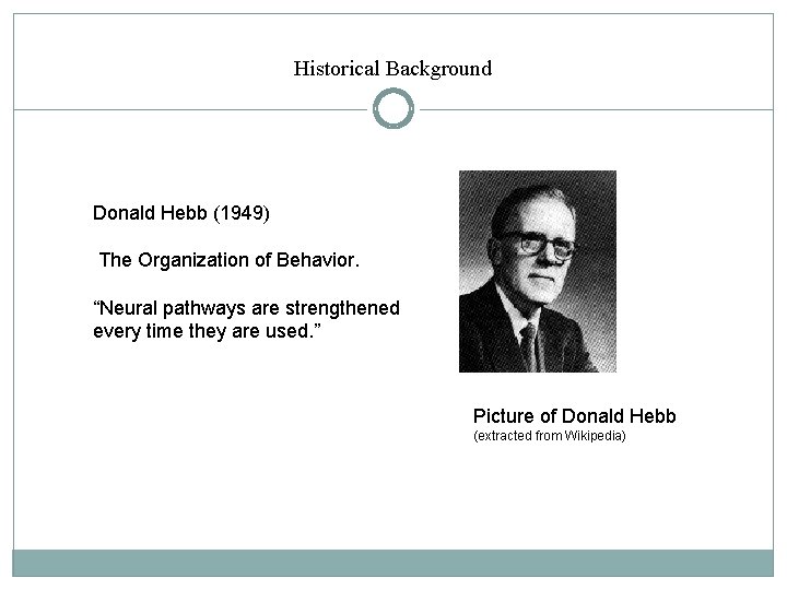
Historical Background Donald Hebb (1949) The Organization of Behavior. “Neural pathways are strengthened every time they are used. ” Picture of Donald Hebb (extracted from Wikipedia)

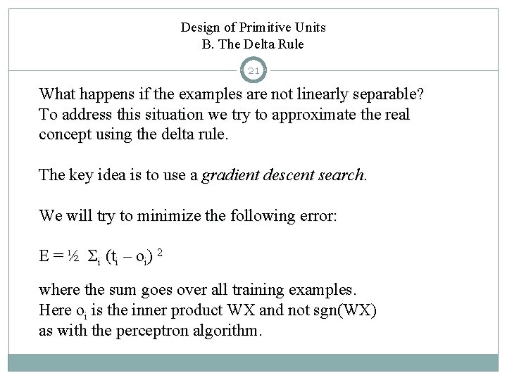
Design of Primitive Units B. The Delta Rule 21 What happens if the examples are not linearly separable? To address this situation we try to approximate the real concept using the delta rule. The key idea is to use a gradient descent search. We will try to minimize the following error: E = ½ Σi (ti – oi) 2 where the sum goes over all training examples. Here oi is the inner product WX and not sgn(WX) as with the perceptron algorithm.

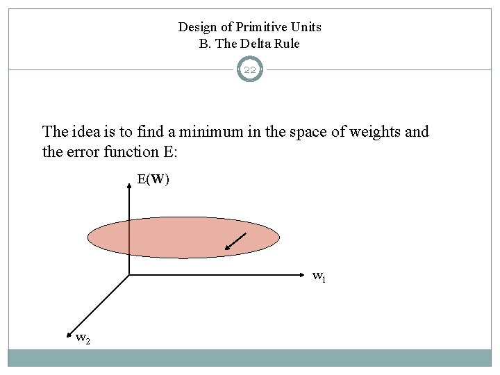
Design of Primitive Units B. The Delta Rule 22 The idea is to find a minimum in the space of weights and the error function E: E(W) w 1 w 2

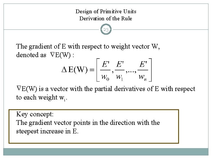
Design of Primitive Units Derivation of the Rule 23 The gradient of E with respect to weight vector W, denoted as E(W) : Δ Δ E(W) is a vector with the partial derivatives of E with respect to each weight wi. Key concept: The gradient vector points in the direction with the steepest increase in E.

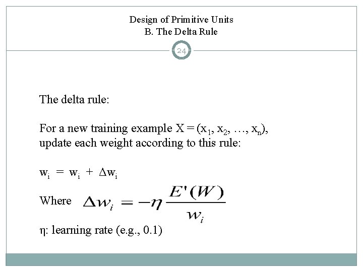
Design of Primitive Units B. The Delta Rule 24 The delta rule: For a new training example X = (x 1, x 2, …, xn), update each weight according to this rule: wi = wi + Δwi Where η: learning rate (e. g. , 0. 1)

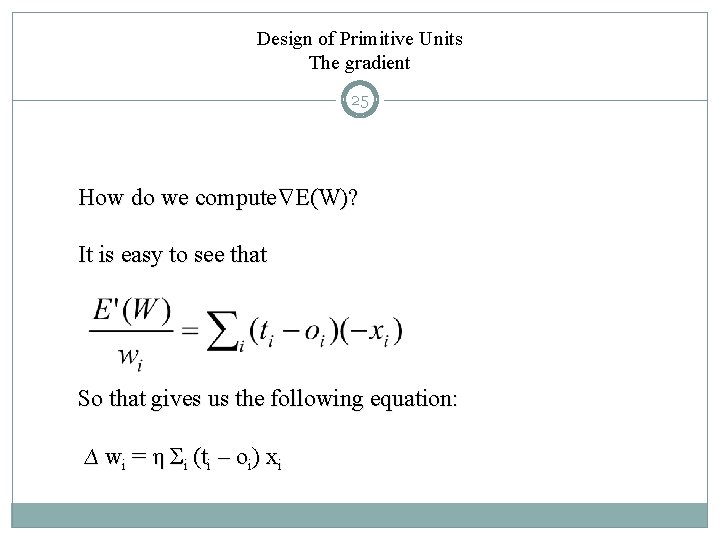
Design of Primitive Units The gradient 25 Δ How do we compute E(W)? It is easy to see that So that gives us the following equation: ∆ wi = η Σi (ti – oi) xi

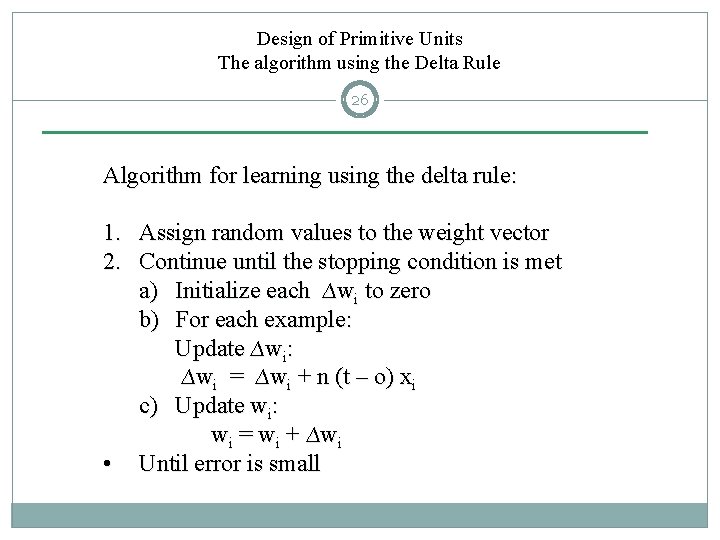
Design of Primitive Units The algorithm using the Delta Rule 26 Algorithm for learning using the delta rule: 1. Assign random values to the weight vector 2. Continue until the stopping condition is met a) Initialize each ∆wi to zero b) For each example: Update ∆wi: ∆wi = ∆wi + n (t – o) xi c) Update wi: wi = wi + ∆wi • Until error is small

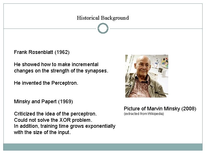
Historical Background Frank Rosenblatt (1962) He showed how to make incremental changes on the strength of the synapses. He invented the Perceptron. Minsky and Papert (1969) Criticized the idea of the perceptron. Could not solve the XOR problem. In addition, training time grows exponentially with the size of the input. Picture of Marvin Minsky (2008) (extracted from Wikipedia)

Design of Primitive Units Difficulties with Gradient Descent 28 There are two main difficulties with the gradient descent method: 1. Convergence to a minimum may take a long time. 2. There is no guarantee we will find the global minimum.

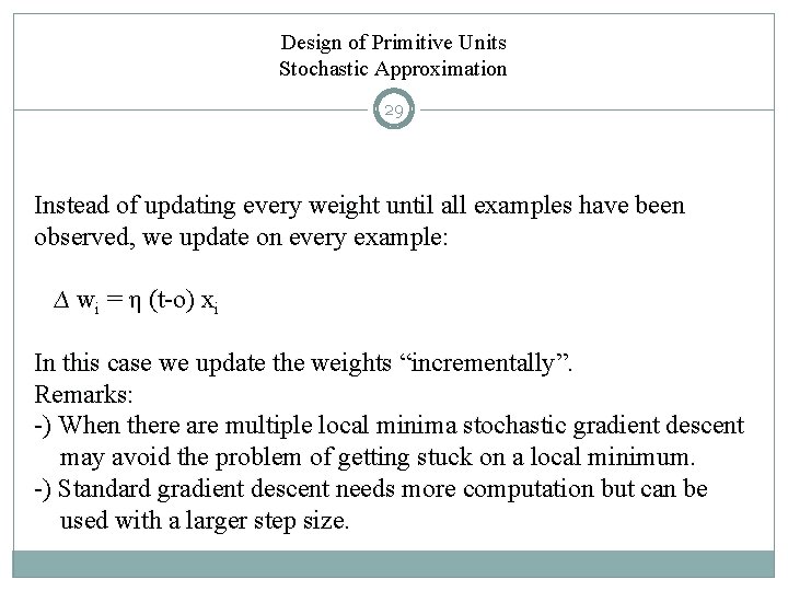
Design of Primitive Units Stochastic Approximation 29 Instead of updating every weight until all examples have been observed, we update on every example: ∆ wi = η (t-o) xi In this case we update the weights “incrementally”. Remarks: -) When there are multiple local minima stochastic gradient descent may avoid the problem of getting stuck on a local minimum. -) Standard gradient descent needs more computation but can be used with a larger step size.

Design of Primitive Units Difference between Perceptron and Delta Rule 30 Ø The perceptron is based on an output from a step function, whereas the delta rule uses the linear combination of inputs directly. Ø The perceptron is guaranteed to converge to a consistent hypothesis assuming the data is linearly separable. The delta rules converges in the limit but it does not need the condition of linearly separable data.