Penalized regression using Lasso All material from Data


 # fit lasso coef(lasso, s=c(1/4, 1/2, 3/4), mode=\"fraction\") #coefficients")
 Gleason score (gleason): scores are assigned to the two")

![prostate <read. csv("C: /Data. Mining/Data/prostate. csv") prostate[1: 3, ] m 1=lm(lcavol~. , data=prostate) summary(m](https://slidetodoc.com/presentation_image_h2/07581a691be0e8956baa7d50d926a119/image-12.jpg "prostate <read. csv(\"C: /Data. Mining/Data/prostate. csv\") prostate[1: 3, ] m 1=lm(lcavol~. , data=prostate) summary(m")
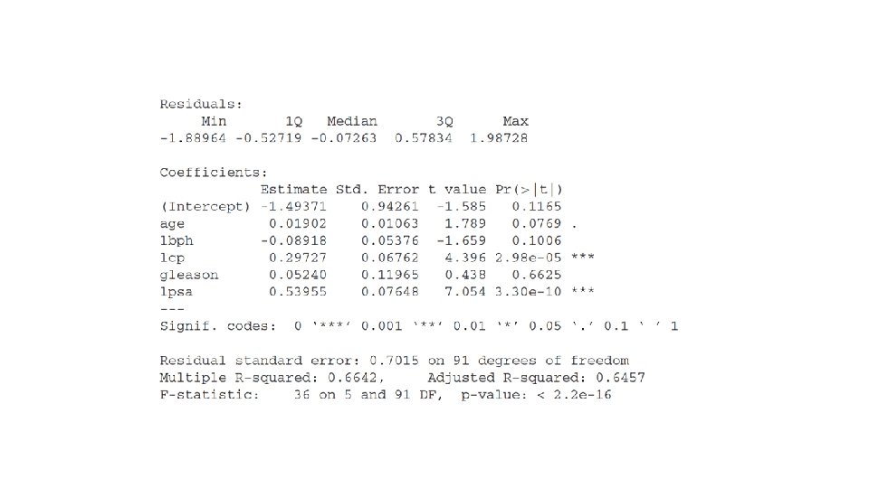

 R-squared: 0. 664")
, mode=\"fraction\") (Intercept) age lbph lcp")
 The output of cross-validation (average mean square errors and their")
- Slides: 19
Penalized regression using Lasso (All material from “Data mining and business analytics with R” by Ledolter)
The L 1 -regularized estimation formulation of the LASSO has a tendency to prefer solutions with fewer nonzero parameter values, thus effectively reducing the number of variables upon which the given solution is dependent. LASSO can be thought of as a penalty-based variable selection approach that selects variables to be included into the model. Such an approach is certainly advantageous in regression situations where one works with extremely large models that contain large number of predictors.
When using the LASSO approach, one needs to select the penalty λ. LASSO estimates are readily obtained for any value of λ. Forecasts can be calculated with the resulting constrained regression estimates, and the out-of-sample prediction performance can be evaluated for any value of λ. This makes cross-validation a very practical approach for selecting the penalty parameter λ. The lars package in R provides LASSO estimates of linear regression coefficients.
The mode = “fraction” argument of this package, with the fraction s representing a number between 0 and 1, provides regression estimates of various degrees of shrinkage. The number s expresses the ratio of the L 1 norm of the LASSO estimate of the coefficient vector, relative to the L 1 norm of the least squares solution. The fraction s = 0, for example, implies that all coefficient estimates are 0 (complete shrinkage to 0); s = 1 leads to the least squares solution.
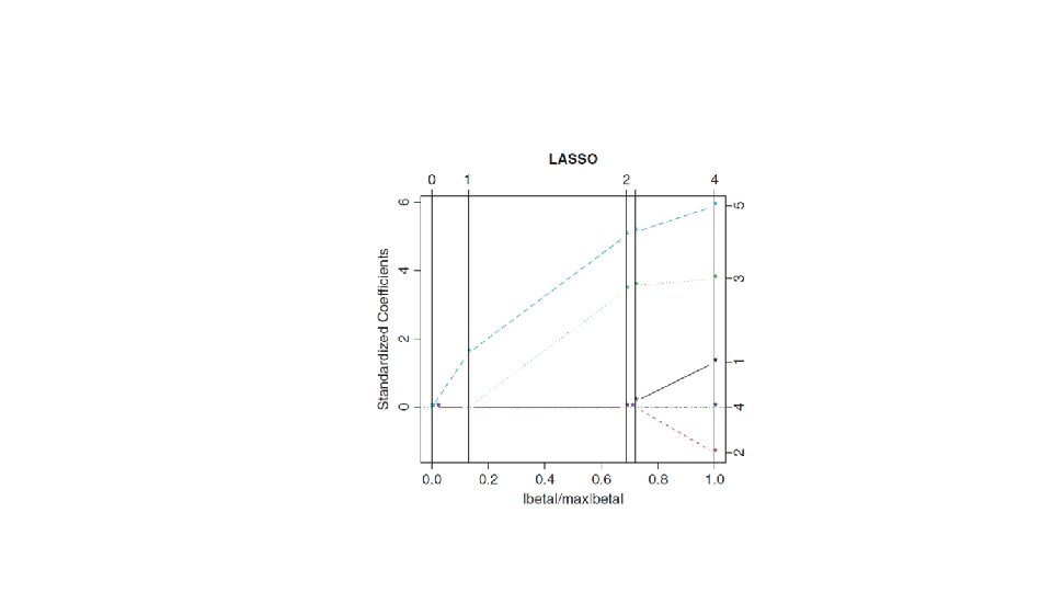
Using the R function plot, one can trace the behavior of the standardized estimates (estimates divided by their standard errors) for changing values of s.
The predict function of the lars library can be used to predict the response with LASSO estimates that have been shrunk to a certain fraction of the least squares estimates. This results in fitted values for in-sample evaluation and in genuine out-of-sample predictions for new cases. The optimal value for s can be obtained through cross-validation and the R command cv. lars.
V-fold cross-validation with K = 10 folds, for example, divides the cases of the data set into K = 10 nonoverlapping parts; it uses 9 of the 10 parts for estimation and the tenth part forecast evaluation. This is repeated 10 times, for the 10 different segments of the holdout sample. Cross -validation mean square errors, plotted for changing values of s, tell us about the shrinkage (the value of s) that should be used.
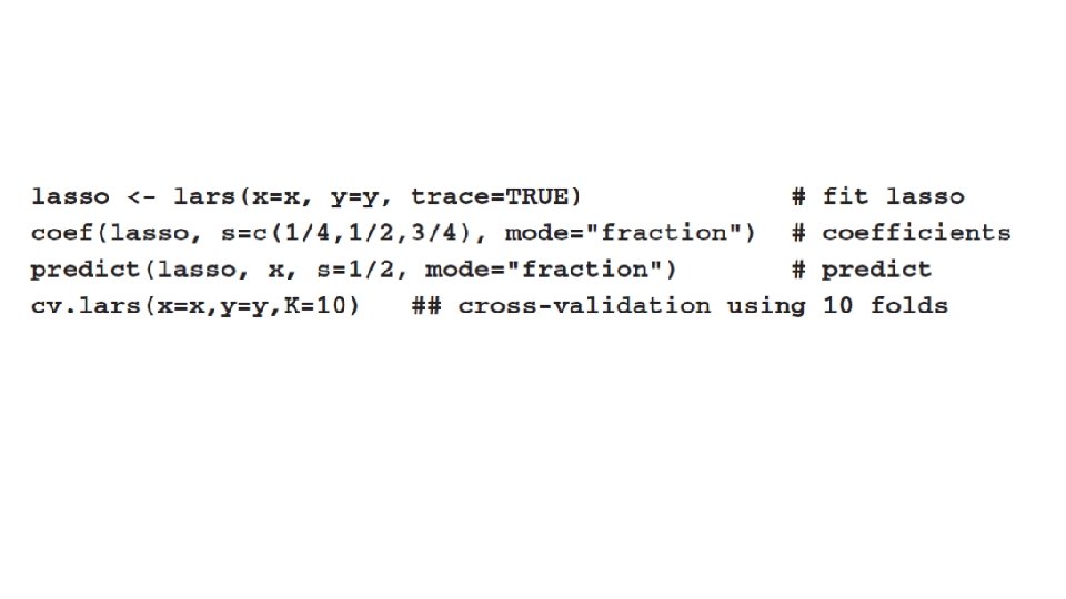
lasso <- lars(x=x, y=y, trace=TRUE) # fit lasso coef(lasso, s=c(1/4, 1/2, 3/4), mode="fraction") #coefficients predict(lasso, x, s=1/2, mode="fraction") # predict cv. lars(x=x, y=y, K=10) ## cross-validation using 10 folds
Prostate Cancer data: (97 patients) Gleason score (gleason): scores are assigned to the two most common tumor patterns ranging from 2 to 10; in this data set, the range is from 6 to 9. Prostate-specific antigen (psa): laboratory results on protein production. Capsular penetration (cp): reach of cancer into the gland lining. Benign prostatic hyperplasia amount (bph): size of the prostate.
The goal is to predict the tumor log volume (which measures the tumor’s size or spread). We try to predict this variable from five covariates (age; logarithms of bph, cp, and psa; and the Gleason score). The predicted size of the tumor has important implications for the subsequent treatment options, which include chemotherapy, radiation treatment, and surgical removal of the prostate.
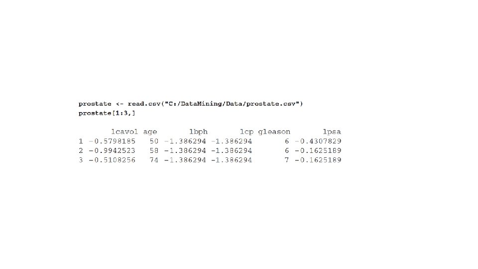
prostate <read. csv("C: /Data. Mining/Data/prostate. csv") prostate[1: 3, ] m 1=lm(lcavol~. , data=prostate) summary(m 1)
## the model. matrix statement defines the model to be fitted x <- model. matrix(lcavol~age+lbph+lcp+gleason+lpsa, + data=prostate) x=x[, -1] ## stripping off the column of 1 s as LASSO includes the ## intercept automatically library(lars) ## lasso on all data lasso <-lars(x=x, y=prostate$lcavol, trace=TRUE) ## trace of lasso (standardized) coefficients for varying ## penalty plot(lasso)
lasso Call: lars(x = x, y = prostate$lcavol, trace = TRUE) R-squared: 0. 664 Sequence of LASSO moves: lpsa lcp age gleason lbph Var 5 3 1 4 2 Step 1 2 3 4 5
coef(lasso, s=c(. 25, . 50, 0. 75, 1. 0), mode="fraction") (Intercept) age lbph lcp gleason lpsa [1, ] 0 0. 000000000 0. 06519506 0. 0000 0. 2128290 # s=0. 25 [2, ] 0 0. 000000000 0. 18564339 0. 0000 0. 3587292 # s=0. 50 [3, ] 0 0. 005369985 -0. 001402051 0. 28821232 0. 01136331 0. 4827810 #s=0. 75 [4, ] 0 0. 019023772 -0. 089182565 0. 29727207 0. 05239529 0. 5395488 #s=1. 00
cv. lars(x=x, y=prostate$lcavol, K=10) The output of cross-validation (average mean square errors and their associated standard error bounds) shows that the mean square error increases quite rapidly if we shrink the coefficients too aggressively. The mean square curve is smallest for s = 1 (the least squares solution), but is actually quite flat for all values of s larger than 0. 6. The present example does not call for much shrinkage. This is not too surprising as the number of estimated coefficients (five coefficients, excluding the intercept) is rather small relative to the size of the sample (n = 97).