PCA SVD Motivation Shape Matching There are tagged

PCA + SVD

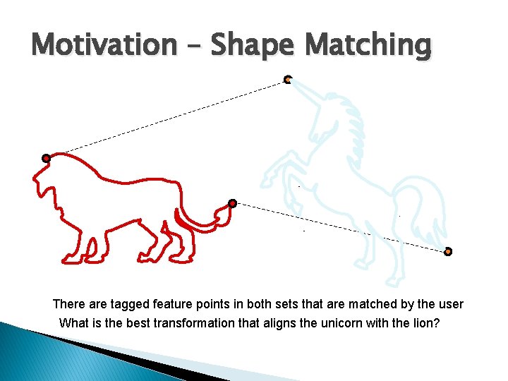
Motivation – Shape Matching There are tagged feature points in both sets that are matched by the user What is the best transformation that aligns the unicorn with the lion?

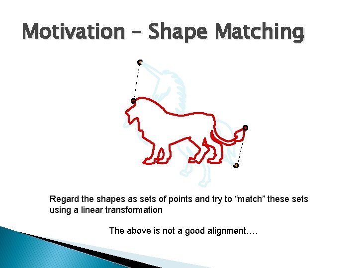
Motivation – Shape Matching Regard the shapes as sets of points and try to “match” these sets using a linear transformation The above is not a good alignment….

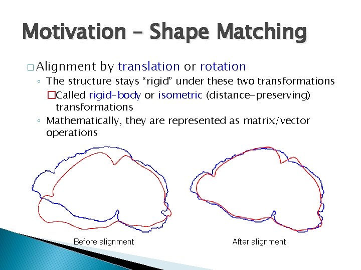
Motivation – Shape Matching � Alignment by translation or rotation ◦ The structure stays “rigid” under these two transformations �Called rigid-body or isometric (distance-preserving) transformations ◦ Mathematically, they are represented as matrix/vector operations Before alignment After alignment

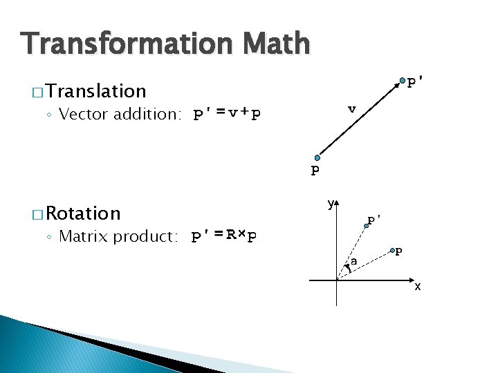
Transformation Math � Translation ◦ Vector addition: � Rotation y ◦ Matrix product: x

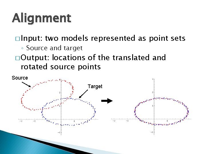
Alignment � Input: two models represented as point sets ◦ Source and target � Output: locations of the translated and rotated source points Source Target

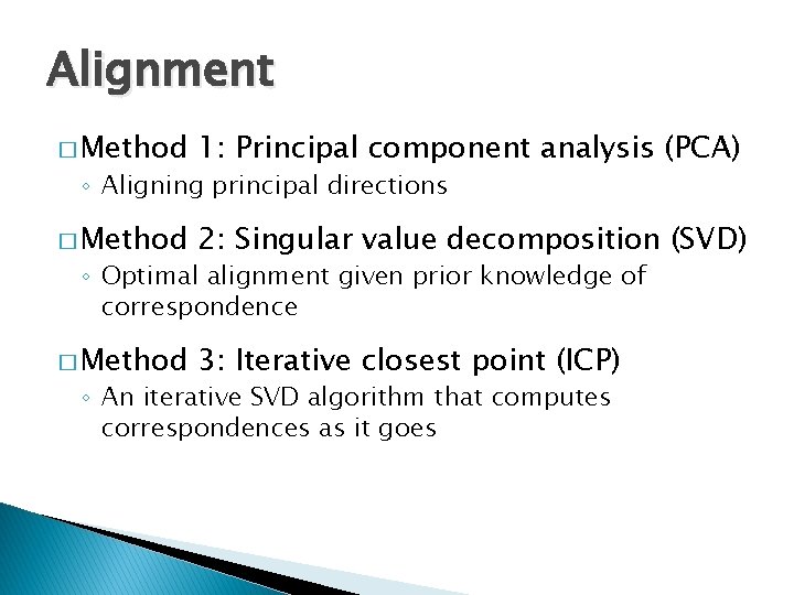
Alignment � Method 1: Principal component analysis (PCA) � Method 2: Singular value decomposition (SVD) � Method 3: Iterative closest point (ICP) ◦ Aligning principal directions ◦ Optimal alignment given prior knowledge of correspondence ◦ An iterative SVD algorithm that computes correspondences as it goes

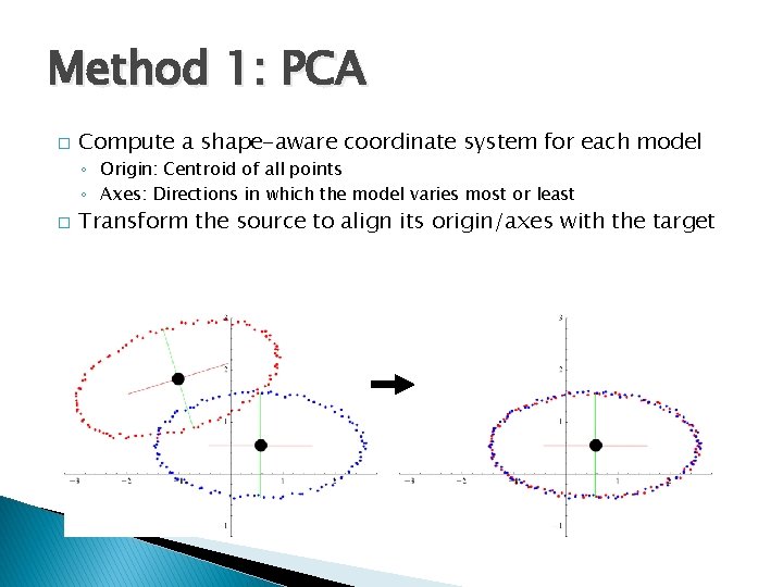
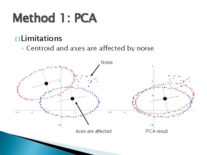
Method 1: PCA � Compute a shape-aware coordinate system for each model ◦ Origin: Centroid of all points ◦ Axes: Directions in which the model varies most or least � Transform the source to align its origin/axes with the target

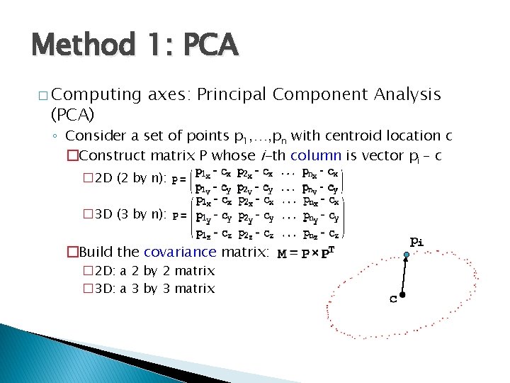
Method 1: PCA � Computing (PCA) axes: Principal Component Analysis ◦ Consider a set of points p 1, …, pn with centroid location c �Construct matrix P whose i-th column is vector pi – c � 2 D (2 by n): � 3 D (3 by n): �Build the covariance matrix: � 2 D: a 2 by 2 matrix � 3 D: a 3 by 3 matrix

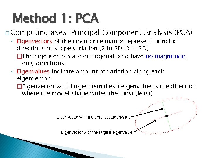
Method 1: PCA � Computing axes: Principal Component Analysis (PCA) ◦ Eigenvectors of the covariance matrix represent principal directions of shape variation (2 in 2 D; 3 in 3 D) �The eigenvectors are orthogonal, and have no magnitude; only directions ◦ Eigenvalues indicate amount of variation along each eigenvector �Eigenvector with largest (smallest) eigenvalue is the direction where the model shape varies the most (least) Eigenvector with the smallest eigenvalue Eigenvector with the largest eigenvalue

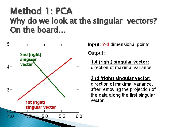
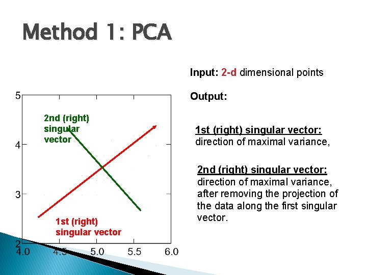
Method 1: PCA Why do we look at the singular vectors? On the board… Input: 2 -d dimensional points 2 nd (right) singular vector 1 st (right) singular vector Output: 1 st (right) singular vector: direction of maximal variance, 2 nd (right) singular vector: direction of maximal variance, after removing the projection of the data along the first singular vector.

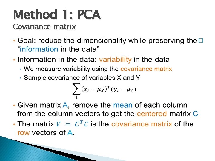
Method 1: PCA Covariance matrix �

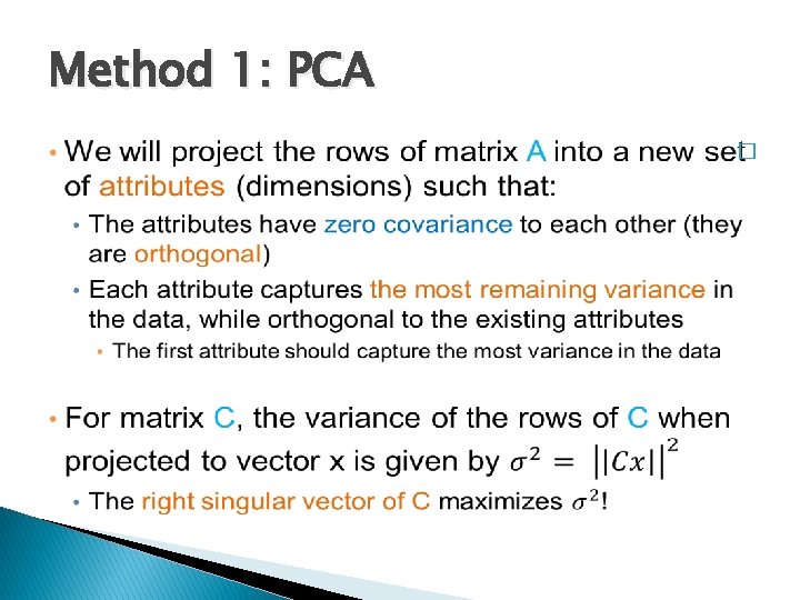
Method 1: PCA �

Method 1: PCA Input: 2 -d dimensional points Output: 2 nd (right) singular vector 1 st (right) singular vector: direction of maximal variance, 2 nd (right) singular vector: direction of maximal variance, after removing the projection of the data along the first singular vector.

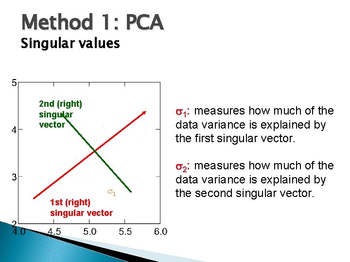
Method 1: PCA Singular values 2 nd (right) singular vector 1: measures how much of the data variance is explained by the first singular vector. 1 1 st (right) singular vector 2: measures how much of the data variance is explained by the second singular vector.

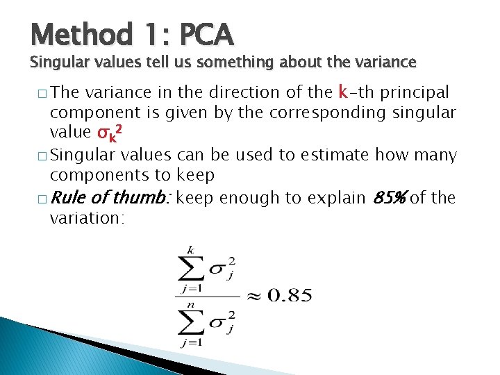
Method 1: PCA Singular values tell us something about the variance � The variance in the direction of the k-th principal component is given by the corresponding singular value σk 2 � Singular values can be used to estimate how many components to keep � Rule of thumb: keep enough to explain 85% of the variation:

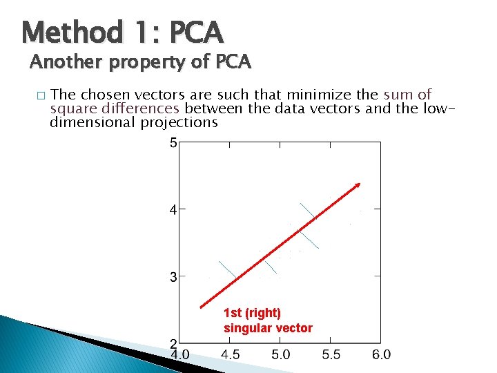
Method 1: PCA Another property of PCA � The chosen vectors are such that minimize the sum of square differences between the data vectors and the lowdimensional projections 1 st (right) singular vector

Method 1: PCA � Limitations ◦ Centroid and axes are affected by noise Noise Axes are affected PCA result

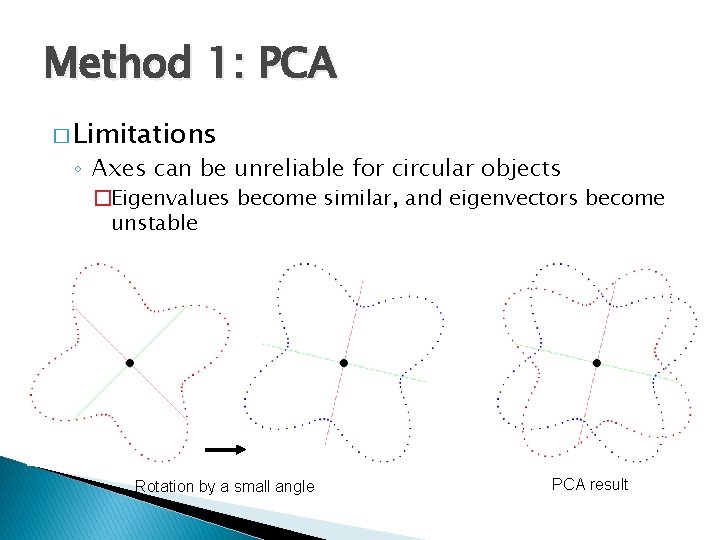
Method 1: PCA � Limitations ◦ Axes can be unreliable for circular objects �Eigenvalues become similar, and eigenvectors become unstable Rotation by a small angle PCA result

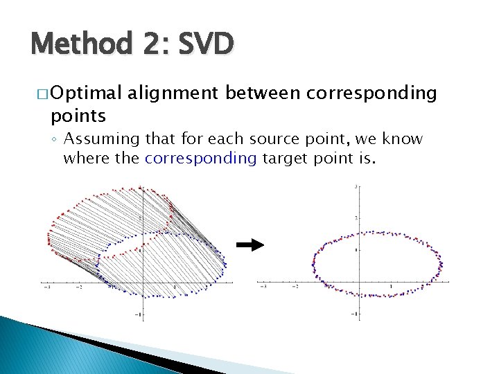
Method 2: SVD � Optimal points alignment between corresponding ◦ Assuming that for each source point, we know where the corresponding target point is.

Method 2: SVD Singular Value Decomposition [n×m] = [n×r] [r×m] r: rank of matrix A U, V are orthogonal matrices

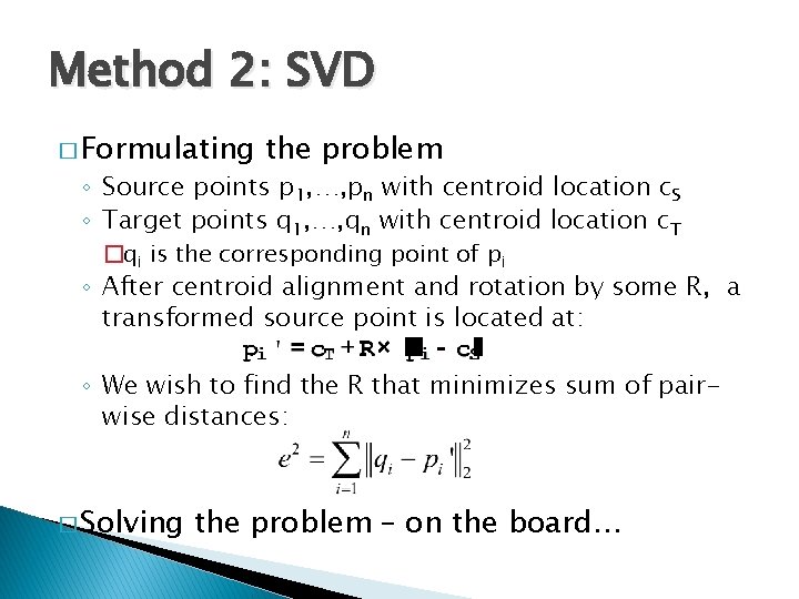
Method 2: SVD � Formulating the problem ◦ Source points p 1, …, pn with centroid location c. S ◦ Target points q 1, …, qn with centroid location c. T �qi is the corresponding point of pi ◦ After centroid alignment and rotation by some R, a transformed source point is located at: ◦ We wish to find the R that minimizes sum of pairwise distances: � Solving the problem – on the board…

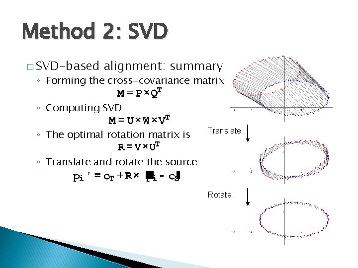
Method 2: SVD � SVD-based alignment: summary ◦ Forming the cross-covariance matrix ◦ Computing SVD ◦ The optimal rotation matrix is Translate ◦ Translate and rotate the source: Rotate

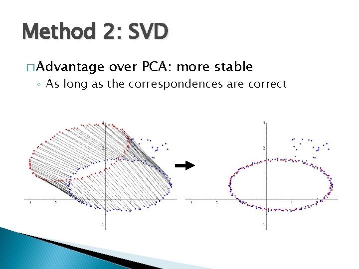
Method 2: SVD � Advantage over PCA: more stable ◦ As long as the correspondences are correct

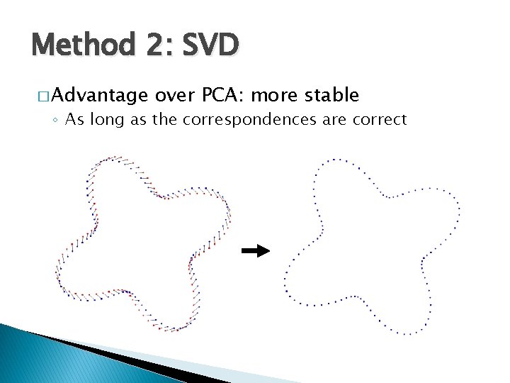
Method 2: SVD � Advantage over PCA: more stable ◦ As long as the correspondences are correct

Method 2: SVD � Limitation: requires accurate correspondences ◦ Which are usually not available

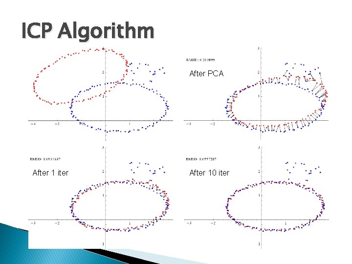
Method 3: ICP � The idea ◦ Use PCA alignment to obtain initial guess of correspondences ◦ Iteratively improve the correspondences after repeated SVD � Iterative closest point (ICP) ◦ 1. Transform the source by PCA-based alignment ◦ 2. For each transformed source point, assign the closest target point as its corresponding point. Align source and target by SVD. �Not all target points need to be used ◦ 3. Repeat step (2) until a termination criteria is met.

ICP Algorithm After PCA After 1 iter After 10 iter

ICP Algorithm After PCA After 1 iter After 10 iter

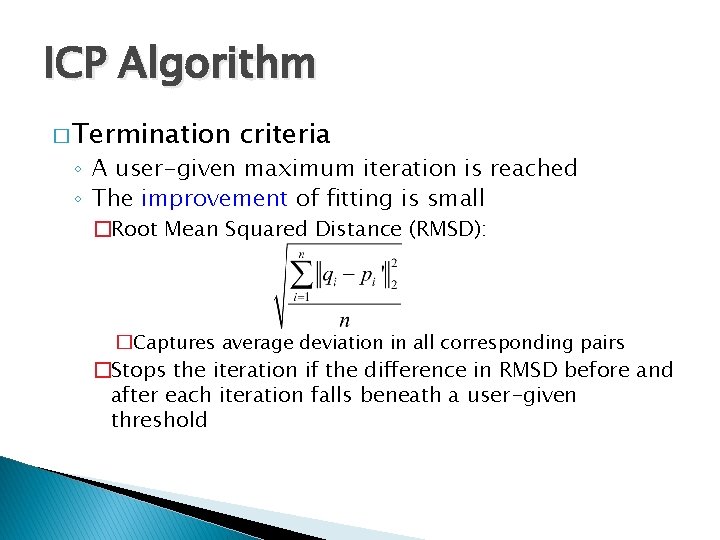
ICP Algorithm � Termination criteria ◦ A user-given maximum iteration is reached ◦ The improvement of fitting is small �Root Mean Squared Distance (RMSD): �Captures average deviation in all corresponding pairs �Stops the iteration if the difference in RMSD before and after each iteration falls beneath a user-given threshold

More Examples After PCA After ICP