Pattern Recognition and Machine LearningChapter 13 Sequential Data

Pattern Recognition and Machine Learning-Chapter 13: Sequential Data Affiliation: Kyoto University Name: Kevin Chien, Dr. Oba Shigeyuki, Dr. Ishii Shin Date: Dec. 9, 2011 1

Idea Origin of Markov Models 2

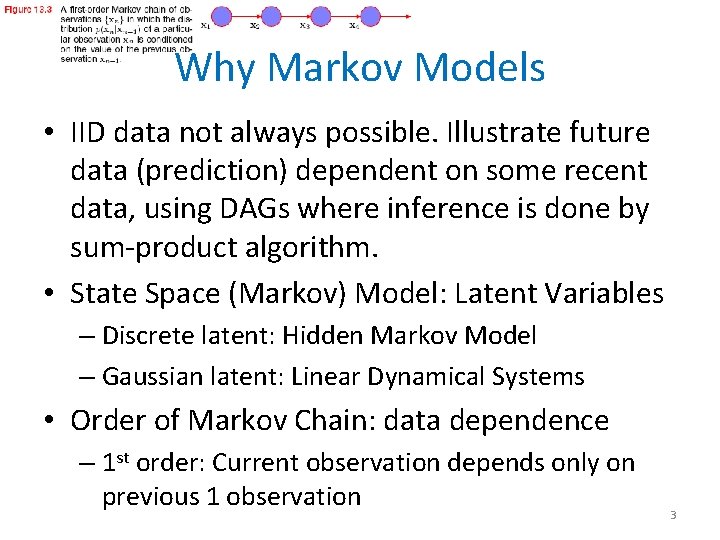
Why Markov Models • IID data not always possible. Illustrate future data (prediction) dependent on some recent data, using DAGs where inference is done by sum-product algorithm. • State Space (Markov) Model: Latent Variables – Discrete latent: Hidden Markov Model – Gaussian latent: Linear Dynamical Systems • Order of Markov Chain: data dependence – 1 st order: Current observation depends only on previous 1 observation 3

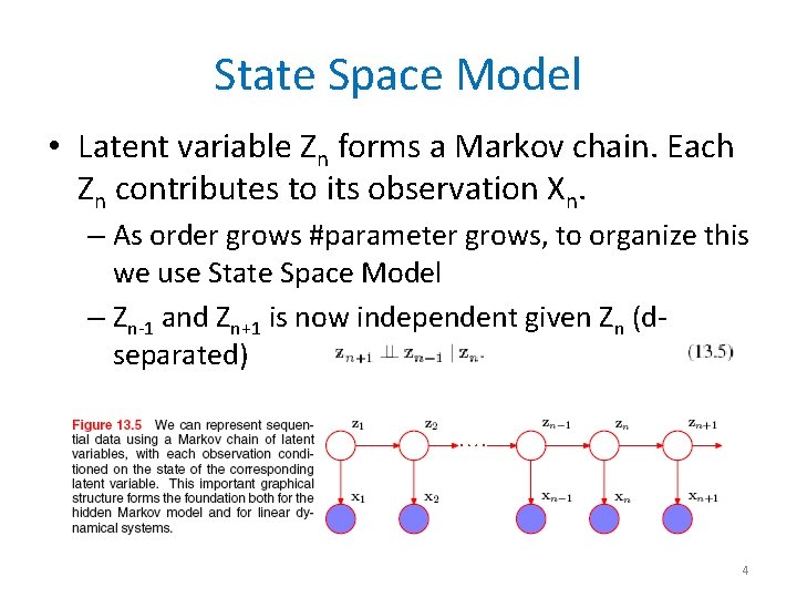
State Space Model • Latent variable Zn forms a Markov chain. Each Zn contributes to its observation Xn. – As order grows #parameter grows, to organize this we use State Space Model – Zn-1 and Zn+1 is now independent given Zn (dseparated) 4

Terminologies For understanding Markov Models 5

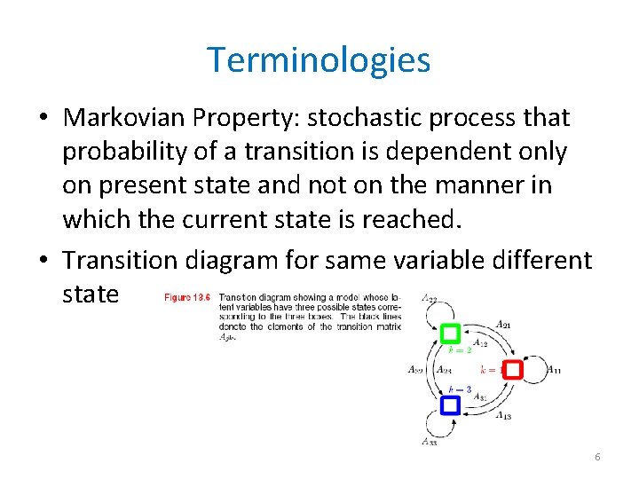
Terminologies • Markovian Property: stochastic process that probability of a transition is dependent only on present state and not on the manner in which the current state is reached. • Transition diagram for same variable different state 6

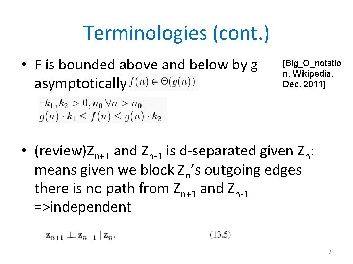
Terminologies (cont. ) • F is bounded above and below by g asymptotically [Big_O_notatio n, Wikipedia, Dec. 2011] • (review)Zn+1 and Zn-1 is d-separated given Zn: means given we block Zn’s outgoing edges there is no path from Zn+1 and Zn-1 =>independent 7

Markov Models Formula and motivation 8

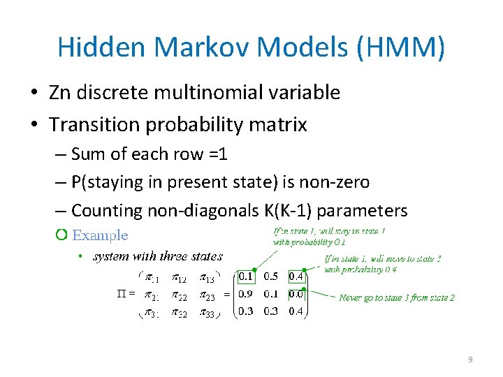
Hidden Markov Models (HMM) • Zn discrete multinomial variable • Transition probability matrix – Sum of each row =1 – P(staying in present state) is non-zero – Counting non-diagonals K(K-1) parameters 9

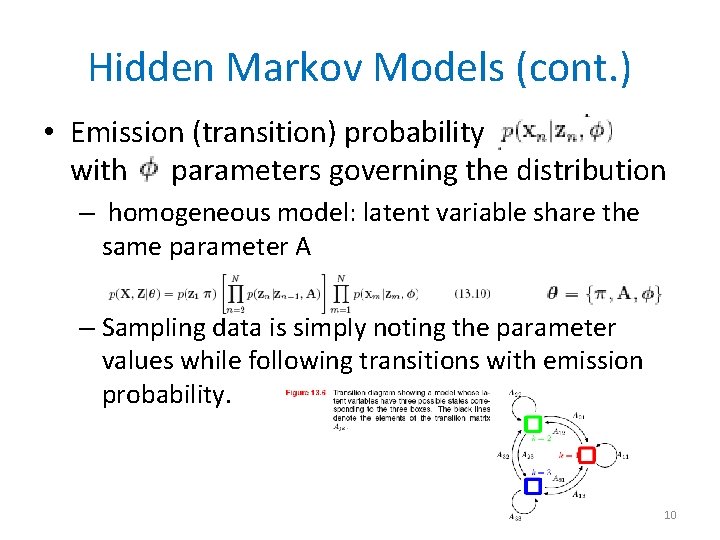
Hidden Markov Models (cont. ) • Emission (transition) probability with parameters governing the distribution – homogeneous model: latent variable share the same parameter A – Sampling data is simply noting the parameter values while following transitions with emission probability. 10

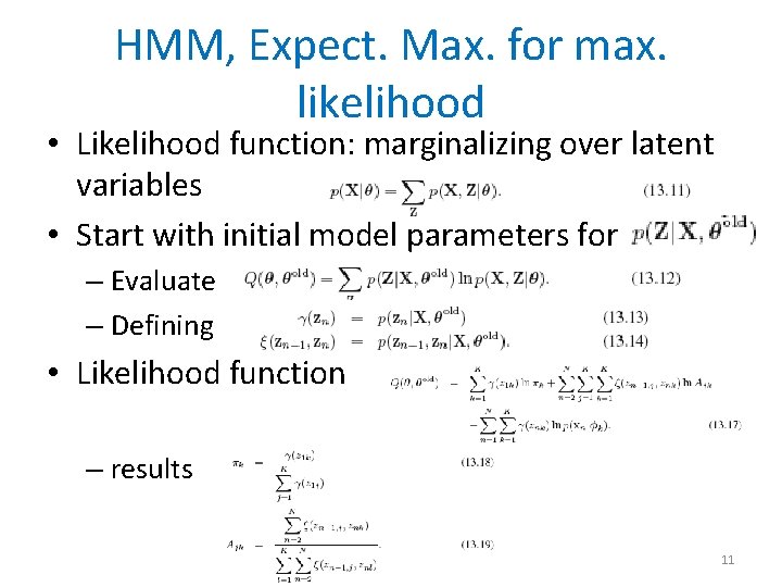
HMM, Expect. Max. for max. likelihood • Likelihood function: marginalizing over latent variables • Start with initial model parameters for – Evaluate – Defining • Likelihood function – results 11

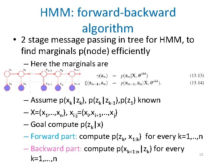
HMM: forward-backward algorithm • 2 stage message passing in tree for HMM, to find marginals p(node) efficiently – Here the marginals are – Assume p(xk|zk), p(zk|zk-1), p(z 1) known – X=(x 1, . . , xn), xi: j=(xi, xi+1, . . , xj) – Goal compute p(zk|x) – Forward part: compute p(zk, x 1: k) for every k=1, . . , n – Backward part: compute p(xk+1: n|zk) for every 12 k=1, …, n

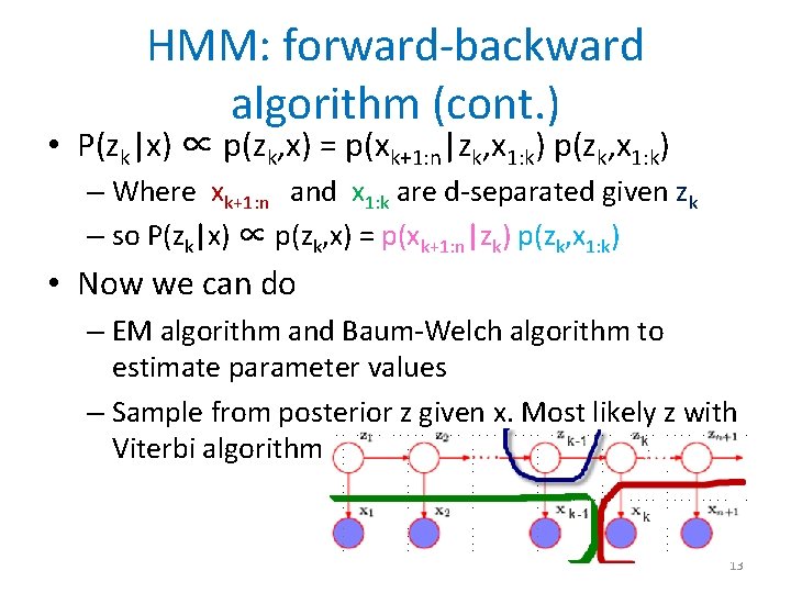
HMM: forward-backward algorithm (cont. ) • P(zk|x) ∝ p(zk, x) = p(xk+1: n|zk, x 1: k) p(zk, x 1: k) – Where xk+1: n and x 1: k are d-separated given zk – so P(zk|x) ∝ p(zk, x) = p(xk+1: n|zk) p(zk, x 1: k) • Now we can do – EM algorithm and Baum-Welch algorithm to estimate parameter values – Sample from posterior z given x. Most likely z with Viterbi algorithm 13

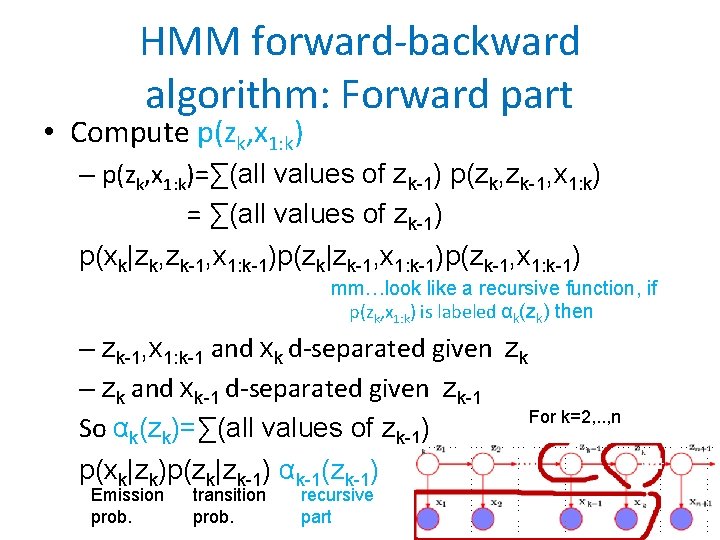
HMM forward-backward algorithm: Forward part • Compute p(zk, x 1: k) – p(zk, x 1: k)=∑(all values of zk-1) p(zk, zk-1, x 1: k) = ∑(all values of zk-1) p(xk|zk, zk-1, x 1: k-1)p(zk|zk-1, x 1: k-1)p(zk-1, x 1: k-1) mm…look like a recursive function, if p(zk, x 1: k) is labeled αk(zk) then – zk-1, x 1: k-1 and xk d-separated given zk – zk and xk-1 d-separated given zk-1 For k=2, . . , n So αk(zk)=∑(all values of zk-1) p(xk|zk)p(zk|zk-1) αk-1(zk-1) Emission prob. transition prob. recursive part 14

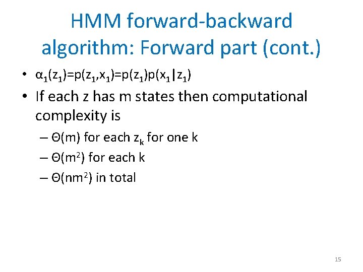
HMM forward-backward algorithm: Forward part (cont. ) • α 1(z 1)=p(z 1, x 1)=p(z 1)p(x 1|z 1) • If each z has m states then computational complexity is – Θ(m) for each zk for one k – Θ(m 2) for each k – Θ(nm 2) in total 15

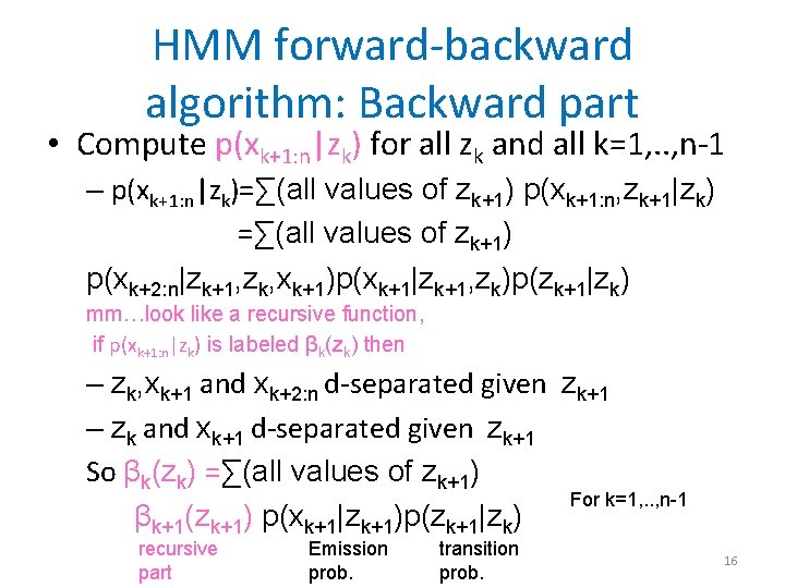
HMM forward-backward algorithm: Backward part • Compute p(xk+1: n|zk) for all zk and all k=1, . . , n-1 – p(xk+1: n|zk)=∑(all values of zk+1) p(xk+1: n, zk+1|zk) =∑(all values of zk+1) p(xk+2: n|zk+1, zk, xk+1)p(xk+1|zk+1, zk)p(zk+1|zk) mm…look like a recursive function, if p(xk+1: n|zk) is labeled βk(zk) then – zk, xk+1 and xk+2: n d-separated given zk+1 – zk and xk+1 d-separated given zk+1 So βk(zk) =∑(all values of zk+1) For k=1, . . , n-1 βk+1(zk+1) p(xk+1|zk+1)p(zk+1|zk) recursive part Emission prob. transition prob. 16

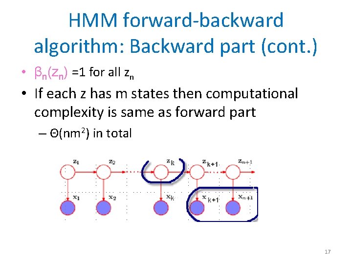
HMM forward-backward algorithm: Backward part (cont. ) • βn(zn) =1 for all zn • If each z has m states then computational complexity is same as forward part – Θ(nm 2) in total 17

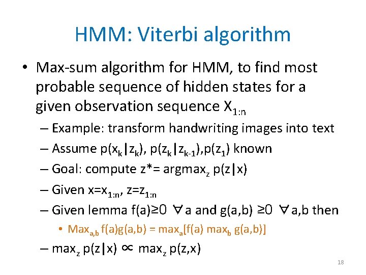
HMM: Viterbi algorithm • Max-sum algorithm for HMM, to find most probable sequence of hidden states for a given observation sequence X 1: n – Example: transform handwriting images into text – Assume p(xk|zk), p(zk|zk-1), p(z 1) known – Goal: compute z*= argmaxz p(z|x) – Given x=x 1: n, z=z 1: n – Given lemma f(a)≥ 0 ∀a and g(a, b) ≥ 0 ∀a, b then • Maxa, b f(a)g(a, b) = maxa[f(a) maxb g(a, b)] – maxz p(z|x) ∝ maxz p(z, x) 18

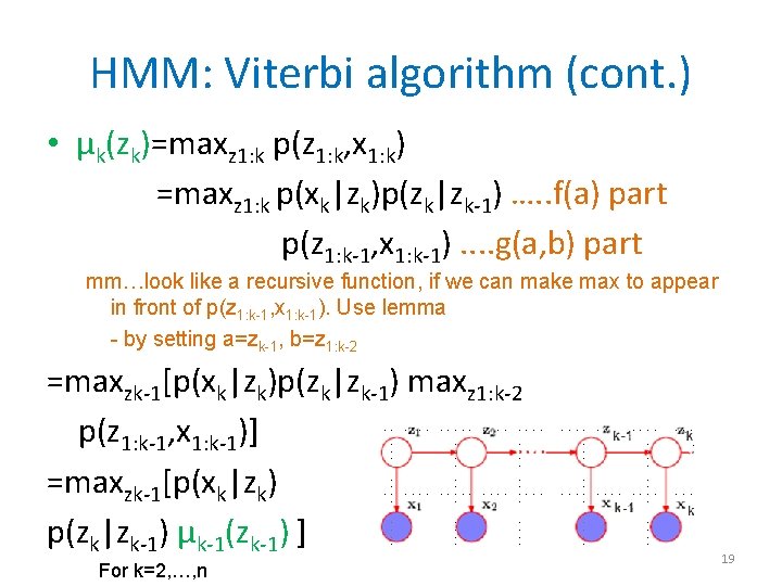
HMM: Viterbi algorithm (cont. ) • μk(zk)=maxz 1: k p(z 1: k, x 1: k) =maxz 1: k p(xk|zk)p(zk|zk-1) …. . f(a) part p(z 1: k-1, x 1: k-1). . g(a, b) part mm…look like a recursive function, if we can make max to appear in front of p(z 1: k-1, x 1: k-1). Use lemma - by setting a=zk-1, b=z 1: k-2 =maxzk-1[p(xk|zk)p(zk|zk-1) maxz 1: k-2 p(z 1: k-1, x 1: k-1)] =maxzk-1[p(xk|zk) p(zk|zk-1) μk-1(zk-1) ] For k=2, …, n 19

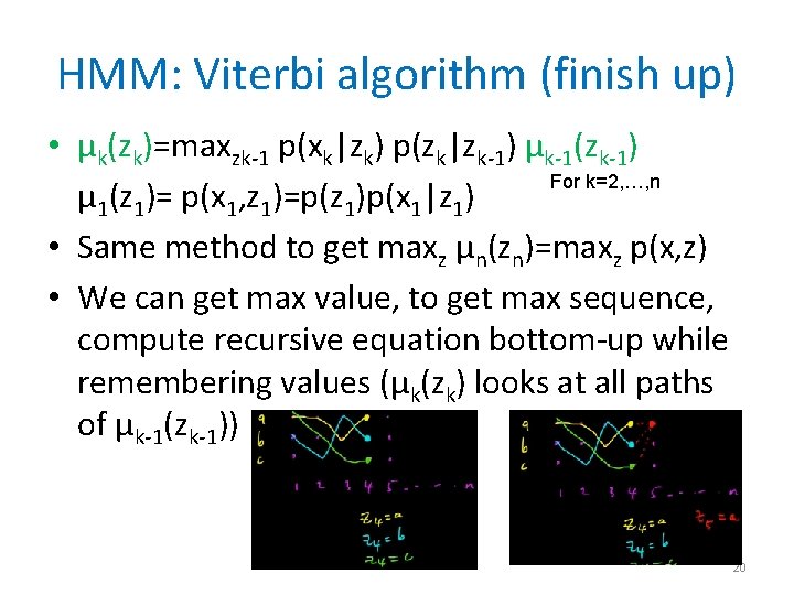
HMM: Viterbi algorithm (finish up) • μk(zk)=maxzk-1 p(xk|zk) p(zk|zk-1) μk-1(zk-1) For k=2, …, n μ 1(z 1)= p(x 1, z 1)=p(z 1)p(x 1|z 1) • Same method to get maxz μn(zn)=maxz p(x, z) • We can get max value, to get max sequence, compute recursive equation bottom-up while remembering values (μk(zk) looks at all paths of μk-1(zk-1)) 20

Additional Information • Excerpt of equations and diagrams from [Pattern Recognition and Machine Learning, Bishop C. M. ] page 605 -646 • Excerpt of equations from Mathematicalmonk, Youtube LLC, Google Inc. , (ML 14. 6 and 14. 7) various titles, July 2011 21