PATTERN RECOGNITION AND MACHINE LEARNING CHAPTER 3 LINEAR

PATTERN RECOGNITION AND MACHINE LEARNING CHAPTER 3: LINEAR MODELS FOR REGRESSION

Outline • • • Discuss tutorial. Regression Examples. The Gaussian distribution. Linear Regression. Maximum Likelihood estimation.

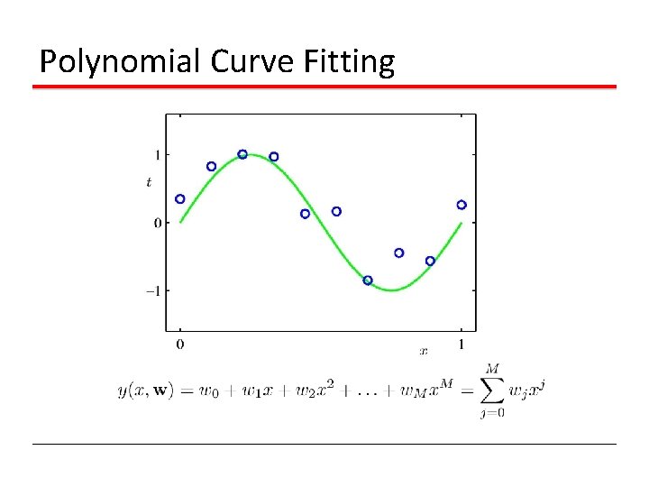
Polynomial Curve Fitting

Academia Example • Predict: final percentage mark for student. • Features: 6 assignment grades, midterm exam, final exam, project, age. • Questions we could ask. • I forgot the weights of components. Can you recover them from a spreadsheet of the final grades? • I lost the final exam grades. How well can I still predict the final mark? • How important is each component, actually? Could I guess well someone’s final mark given their assignments? Given their exams?

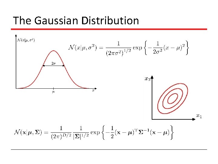
The Gaussian Distribution

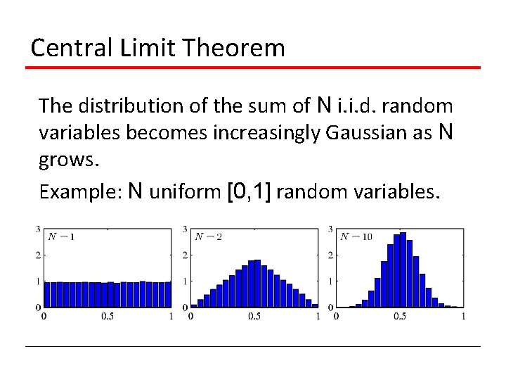
Central Limit Theorem The distribution of the sum of N i. i. d. random variables becomes increasingly Gaussian as N grows. Example: N uniform [0, 1] random variables.

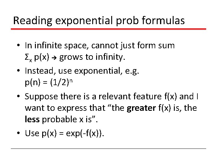
Reading exponential prob formulas • In infinite space, cannot just form sum Σx p(x) grows to infinity. • Instead, use exponential, e. g. p(n) = (1/2)n • Suppose there is a relevant feature f(x) and I want to express that “the greater f(x) is, the less probable x is”. • Use p(x) = exp(-f(x)).

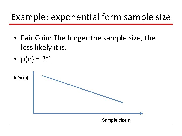
Example: exponential form sample size • Fair Coin: The longer the sample size, the less likely it is. • p(n) = 2 -n. ln[p(n)] Sample size n

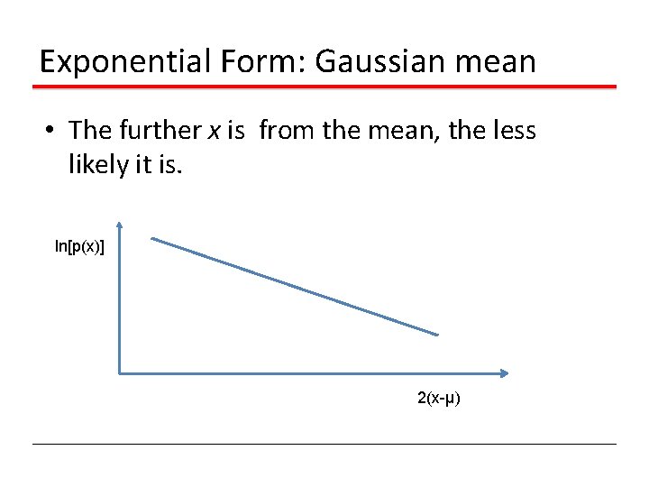
Exponential Form: Gaussian mean • The further x is from the mean, the less likely it is. ln[p(x)] 2(x-μ)

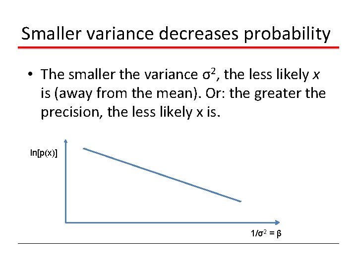
Smaller variance decreases probability • The smaller the variance σ2, the less likely x is (away from the mean). Or: the greater the precision, the less likely x is. ln[p(x)] 1/σ2 = β

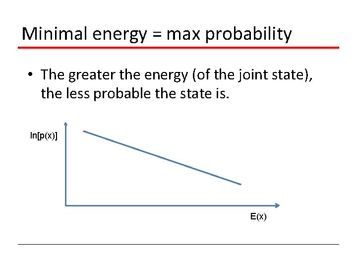
Minimal energy = max probability • The greater the energy (of the joint state), the less probable the state is. ln[p(x)] E(x)

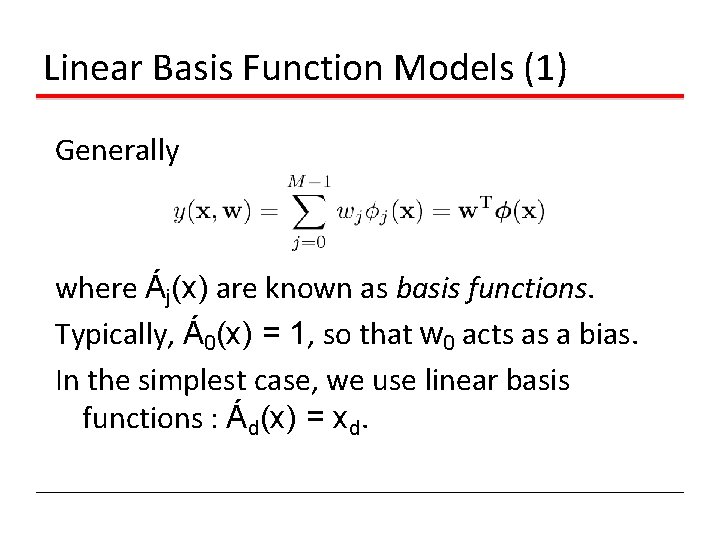
Linear Basis Function Models (1) Generally where Áj(x) are known as basis functions. Typically, Á0(x) = 1, so that w 0 acts as a bias. In the simplest case, we use linear basis functions : Ád(x) = xd.

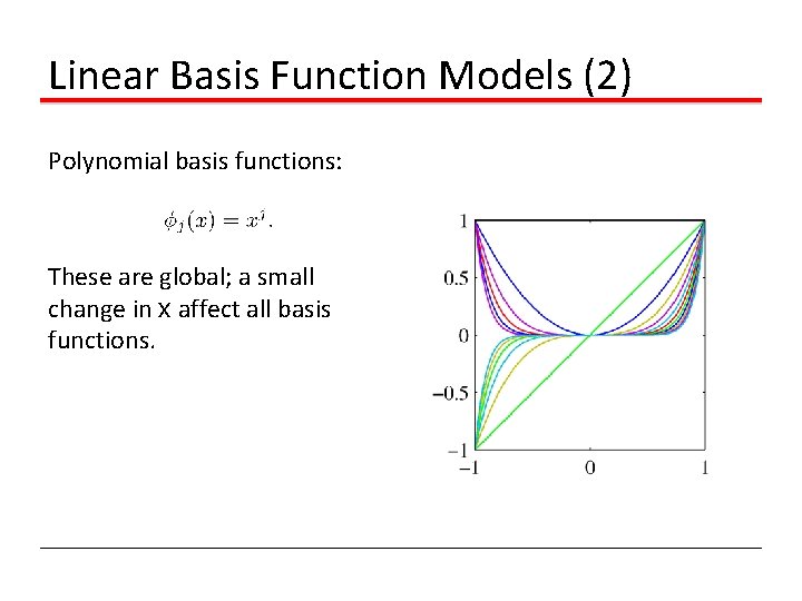
Linear Basis Function Models (2) Polynomial basis functions: These are global; a small change in x affect all basis functions.

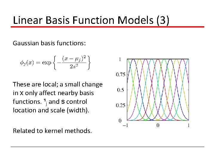
Linear Basis Function Models (3) Gaussian basis functions: These are local; a small change in x only affect nearby basis functions. ¹j and s control location and scale (width). Related to kernel methods.

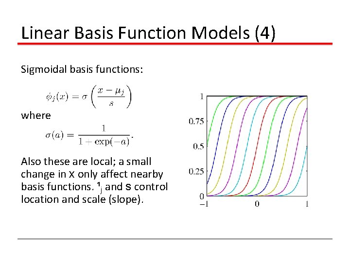
Linear Basis Function Models (4) Sigmoidal basis functions: where Also these are local; a small change in x only affect nearby basis functions. ¹j and s control location and scale (slope).

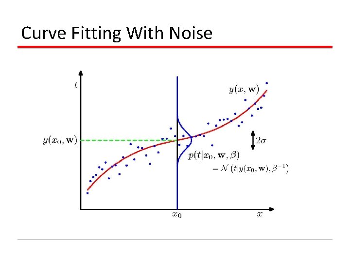
Curve Fitting With Noise

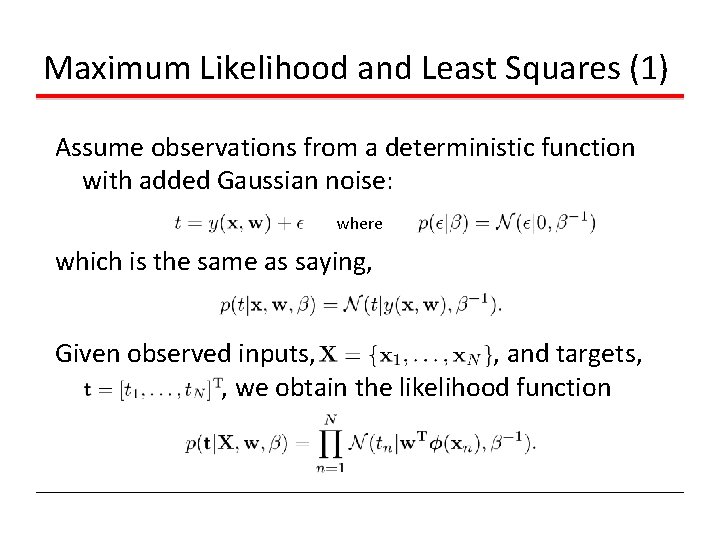
Maximum Likelihood and Least Squares (1) Assume observations from a deterministic function with added Gaussian noise: where which is the same as saying, Given observed inputs, , and targets, , we obtain the likelihood function

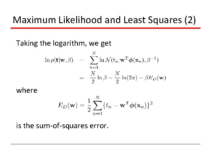
Maximum Likelihood and Least Squares (2) Taking the logarithm, we get where is the sum-of-squares error.

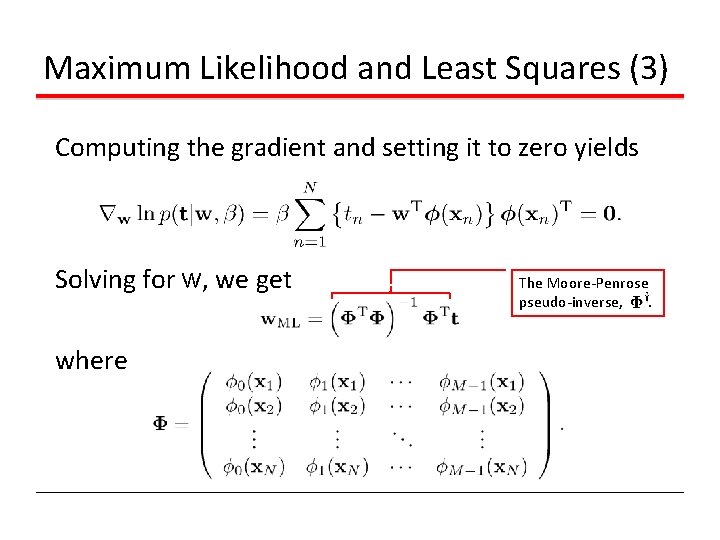
Maximum Likelihood and Least Squares (3) Computing the gradient and setting it to zero yields Solving for w, we get where The Moore-Penrose pseudo-inverse, .

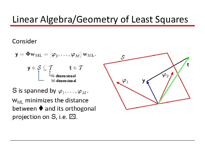
Linear Algebra/Geometry of Least Squares Consider N-dimensional M-dimensional S is spanned by. w. ML minimizes the distance between t and its orthogonal projection on S, i. e. y.

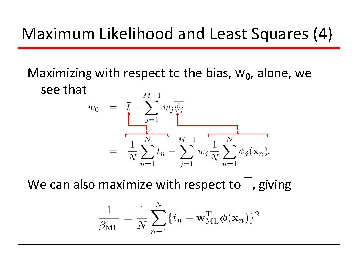
Maximum Likelihood and Least Squares (4) Maximizing with respect to the bias, w 0, alone, we see that We can also maximize with respect to ¯, giving

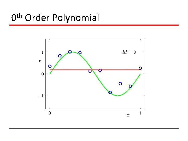
0 th Order Polynomial

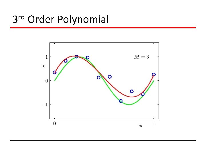
3 rd Order Polynomial

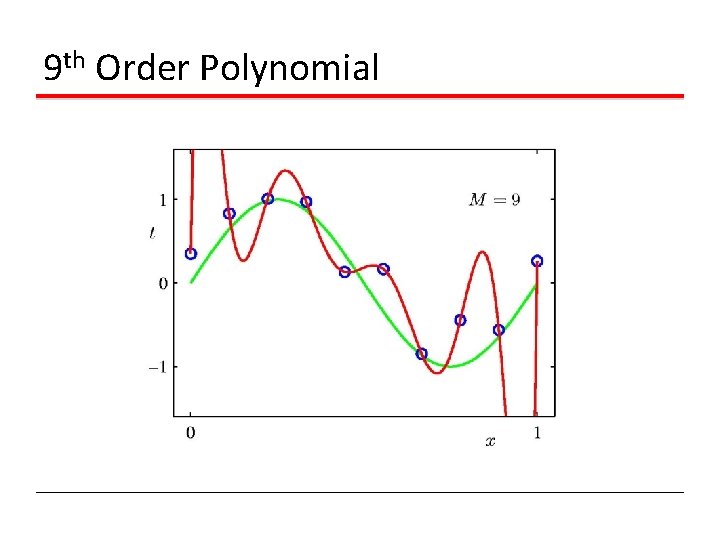
9 th Order Polynomial

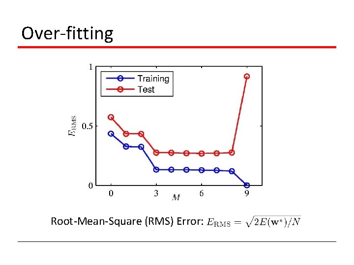
Over-fitting Root-Mean-Square (RMS) Error:

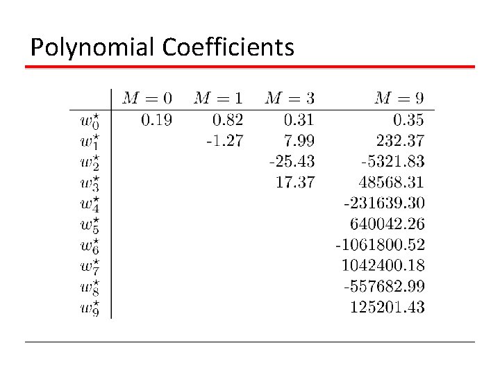
Polynomial Coefficients

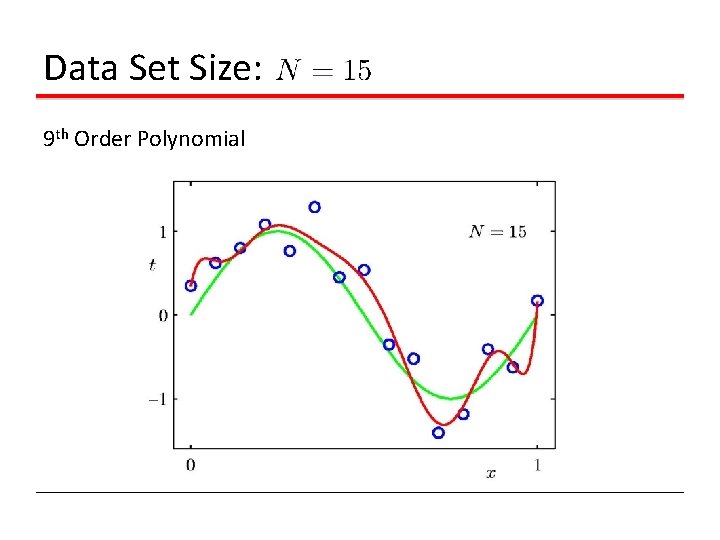
Data Set Size: 9 th Order Polynomial

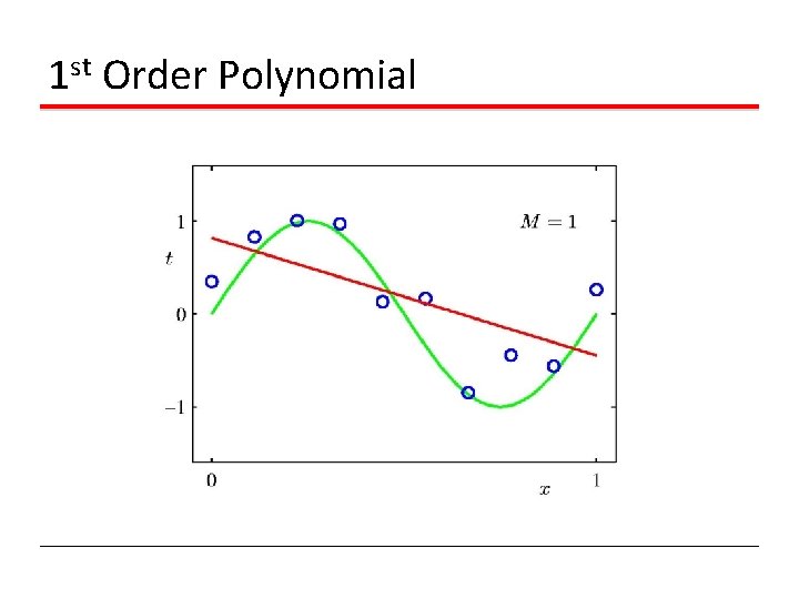
1 st Order Polynomial

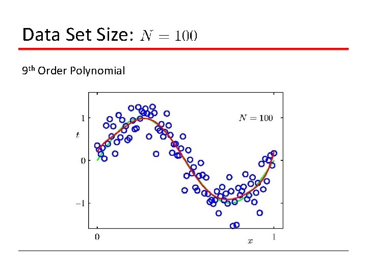
Data Set Size: 9 th Order Polynomial

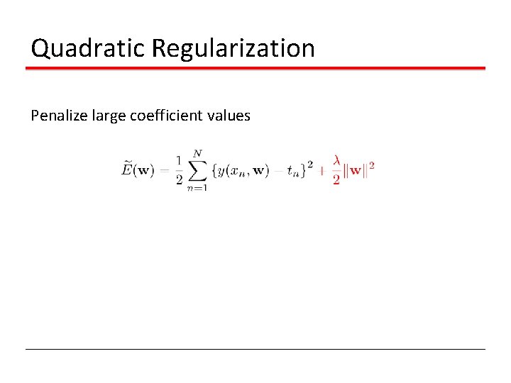
Quadratic Regularization Penalize large coefficient values

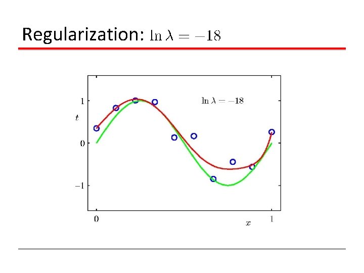
Regularization:

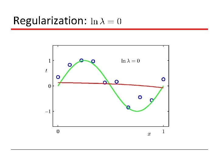
Regularization:

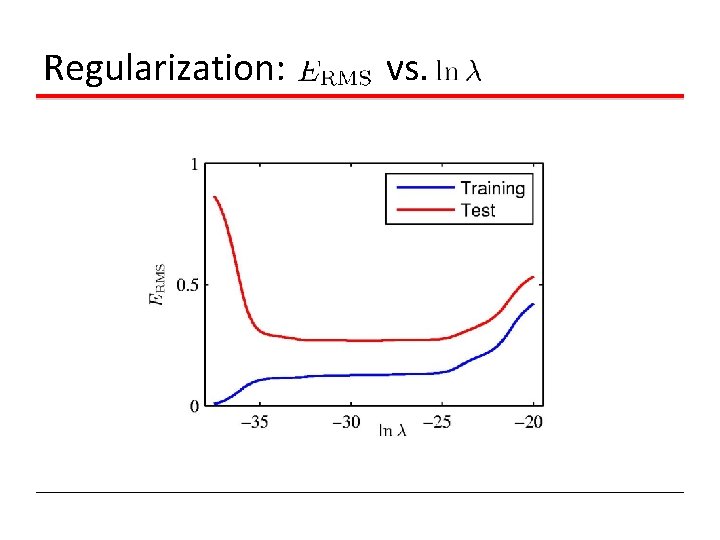
Regularization: vs.

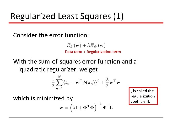
Regularized Least Squares (1) Consider the error function: Data term + Regularization term With the sum-of-squares error function and a quadratic regularizer, we get which is minimized by ¸ is called the regularization coefficient.

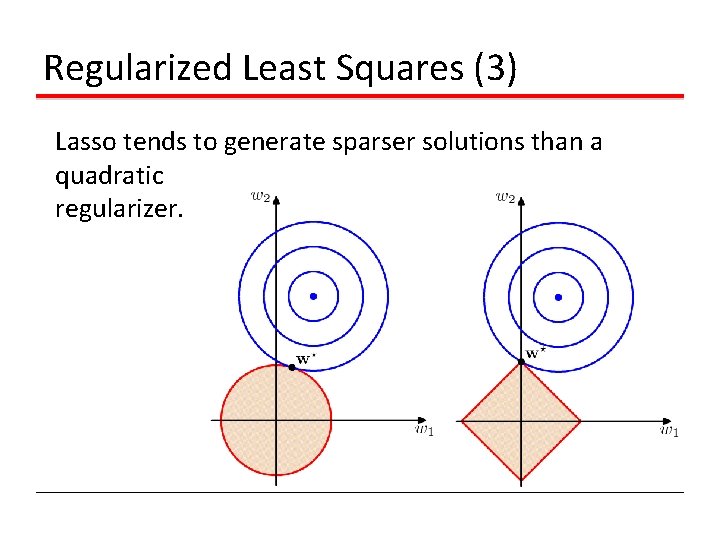
Regularized Least Squares (2) With a more general regularizer, we have Lasso Quadratic

Regularized Least Squares (3) Lasso tends to generate sparser solutions than a quadratic regularizer.

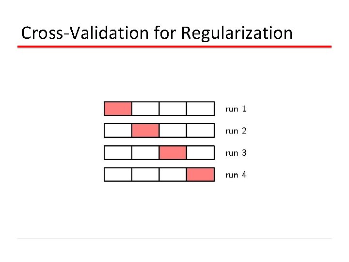
Cross-Validation for Regularization

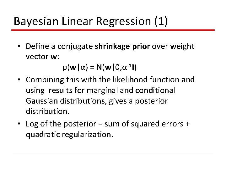
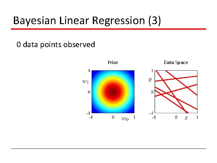
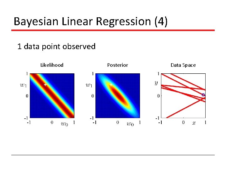
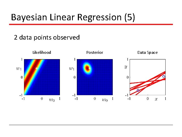
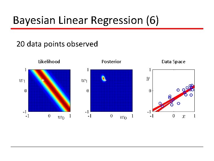
Bayesian Linear Regression (1) • Define a conjugate shrinkage prior over weight vector w: p(w|α) = N(w|0, α-1 I) • Combining this with the likelihood function and using results for marginal and conditional Gaussian distributions, gives a posterior distribution. • Log of the posterior = sum of squared errors + quadratic regularization.

Bayesian Linear Regression (3) 0 data points observed Prior Data Space

Bayesian Linear Regression (4) 1 data point observed Likelihood Posterior Data Space

Bayesian Linear Regression (5) 2 data points observed Likelihood Posterior Data Space

Bayesian Linear Regression (6) 20 data points observed Likelihood Posterior Data Space

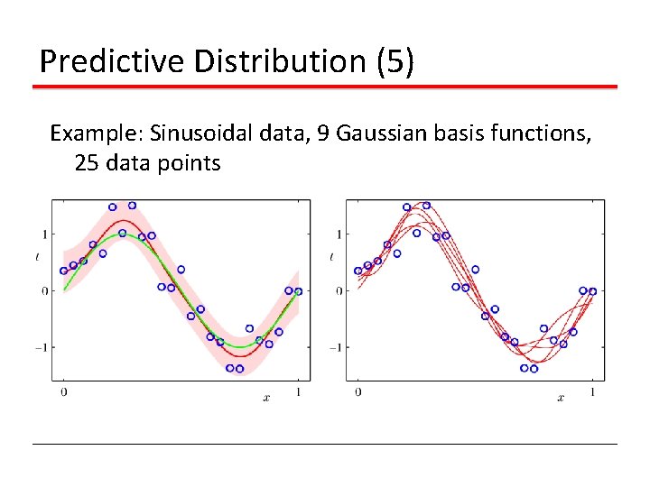
Predictive Distribution (1) • Predict t for new values of x by integrating over w. • Can be solved analytically.

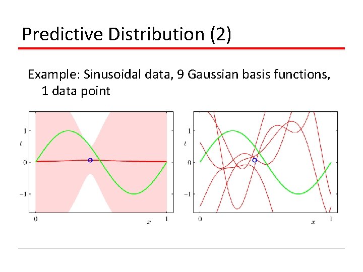
Predictive Distribution (2) Example: Sinusoidal data, 9 Gaussian basis functions, 1 data point

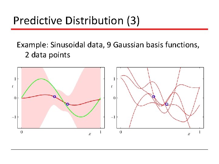
Predictive Distribution (3) Example: Sinusoidal data, 9 Gaussian basis functions, 2 data points

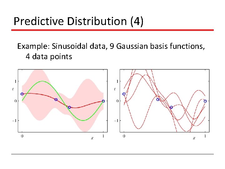
Predictive Distribution (4) Example: Sinusoidal data, 9 Gaussian basis functions, 4 data points

Predictive Distribution (5) Example: Sinusoidal data, 9 Gaussian basis functions, 25 data points

Limitations of Fixed Basis Functions • M basis function along each dimension of a D-dimensional input space requires MD basis functions: the curse of dimensionality. • In later chapters, we shall see how we can get away with fewer basis functions, by choosing these using the training data.