Pattern Recognition and Image Analysis Dr Manal Helal

Pattern Recognition and Image Analysis Dr. Manal Helal – Fall 2014 Lecture 4

Parameter Estimations 2

Course Outline MODEL INFORMATION COMPLETE Bayes Decision Theory Parametric Approach “Optimal” Plug-in Rules INCOMPLETE Supervised Learning Nonparametric Approach Unsupervised Learning Parametric Approach Density Geometric Rules Estimation (K-NN, MLP) Mixture Resolving Nonparametric Approach Cluster Analysis (Hard, Fuzzy)

4 We know very little n The ultimate goal of all sciences is to arrive at quantitative models that describe nature with a sufficient accuracy - or to put it short: to calculate nature. These calculations have the general form answer = f (question) or output = f (input) n Laws of nature is rather limited (although expanding) to answer all questions. n Chemists, material’s scientists, engineers or biologists who want to ask questions like the biological effect of a new molecular entity or the properties of a new material’s composition, will require to estimate some parameters from what they know.

5 To Expand our knowledge n Situation 1: The model function f is theoretically or empirically known. Then the output quantity of interest may be calculated directly. n Situation 2: The structural form of the function f is known but not the values of its parameters. Then these parameter values may be statistically estimated on the basis of experimental data by curve fitting methods. n Situation 3: Even the structural form of the function f is unknown. As an approximation the function f may be modeled by a machine learning technique on the basis of experimental data.

6 Situation 2 – 2 D n Input x produces output y linearly according to the line equation: y= f(x)=b 1+b 2 x n b 1 and b 2 parameters of this line, (y-intercept of the line and the slope) can be estimates geometrically, or by curve fitting, using least squares method.

Situation 2 – Higher Dimensions Chikazoe, J, Lee H, Kriegeskorte N, & Anderson A, “Population coding of affect across stimuli, modalities and individuals”, Nature Neuroscience 17, 111 4– 1122 (2014) Received 19 January 2014 Accepted 23 May 2014 Published online 22 June 2014 7

(a) ROIs were determined on the basis of anatomical gray matter masks. (b) The 128 visual scene stimuli were arranged using MDS such that pairwise distances reflected neural response-pattern similarity. Color code indicates feature magnitude scores for low-level visual features in EVC (top), animacy in VTC (middle) and subjective valence in OFC (bottom) for the same stimuli. Examples i, iii, iv and v traverse the primary dimension in each feature space, with pictures illustrating visual features (for example, luminance) (top), animacy (middle) and valence (bottom).

9 Limitations n More than 10 dimensions, difficult to visualise without transformations, n Situation 3 is most difficult

10 Parametric Distributions n Parametric distributions are probability distributions that you can describe using a finite set of parameters. 1. You can choose a distribution model for your data based on a parametric family of probability distributions, 2. then adjust the parameters to fit the data. 3. You can then perform further analyses by computing summary statistics, evaluating the probability density function (pdf) and cumulative distribution function (cdf), and assessing the fit of the distribution to your data.

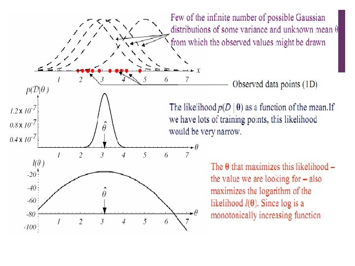
11 Parameter Estimation n When seen from a distance, without prior knowledge about how many girls and boys, we might see a : Boy or Girl n We denote by θ the (unknown) probability P(B). n Estimation task: n Given a sequence of students, x[1], x[2], . . . , x[M] we want to estimate the probabilities P(B)= θ and P(G) = 1 - θ

12 n n Consider instances x[1], x[2], . . . , x[M] such that n The set of values that x can take is known n Each is sampled from the same distribution n Each sampled independently of the rest Here we focus on multinomial distributions n Only finitely many possible values for x n Special case: binomial, with values B(oy) and G(irl)

Two major approaches n n Maximum-Likelihood Method Bayesian Method n Use P( i | x) for our classification rule! n Results are nearly identical, but the approaches are different

Maximum-Likelihood vs. Bayesian: l l Maximum Likelihood n Parameters are fixed but unknown! n Best parameters are obtained by maximizing the probability of obtaining the samples observed Bayes Parameters are random variables having some known distribution n Best parameters are obtained by estimating them given the new data, converts the prior to a posterior density. n

15 Maximum-Likelihood Estimation n Has good convergence properties as the sample size increases n Simpler than any other alternative techniques n Principles: n Choose parameters that maximize the likelihood function n This is one of the most commonly used estimators in statistics n Intuitively appealing 2

16 Major assumptions n Suppose we have a set D = {x 1, . . . , xn} of independent and identically distributed (i. i. d. ) samples drawn from the density p(x|θ). n We would like to use training samples in D to estimate the unknown parameter vector θ. n Define L(θ|D) as the likelihood function of θ with respect to D as 1

17 n The maximum likelihood estimate (MLE) of θ is, by definition, the value that maximizes L(θ|D) and can be computed as n It is often easier to work with the logarithm of the likelihood function (log-likelihood function) that gives

18 The Binomial Likelihood Function n How good is a particular θ? It depends on how likely it is to generate the observed data n L(θ: D) = P(D|θ) = ∏P(x[m]|θ) m n The likelihood for the sequence B, G, G, B, B is L(θ: D) = θ⋅(1−θ)⋅θ⋅θ

19 Example: MLE in Binomial Data n It can be shown that the MLE for the probability of boys is given by n which coincides with what one would expect n Example: (NB, NG ) = (3, 2) n MLE estimate is 3/5 = 0. 6

20 From Binomial to Multinomial n For example, suppose X can have the values 1, 2, . . . , K n We want to learn the parameters θ 1, θ 2. . , θ K Observations: n N 1, N 2, . . . , NK - the number of times each outcome is observed n Likelihood n MLE function:

22 Maximum Likelihood Estimation n If the number of parameters is p, i. e. , θ = (θ 1, . . . , θp)T , define the gradient operator n Then, the MLE of θ should satisfy the necessary conditions

23 Maximum Likelihood Estimation n Properties of MLEs: n �� The MLE is the parameter point for which the observed sample is the most likely. n �� The procedure with partial derivatives may result in several local extrema. We should check each solution individually to identify the global optimum. n �� Boundary conditions must also be checked separately extrema. for n �� Invariance property: if the MLE of f(θ) is f( ). isθ, then. MLE for of any function f(θ),

Bayes Parameter Estimation 24

Bayesian Estimation q are random variables that have some known a-priori distribution p(q). n Estimates a distribution rather than making point estimates like ML. n Assumes that the parameters BE solution might not be of the parametric form assumed.

Bayesian Estimation (BE) • Need to estimate p(x/ωi, Di) for every class ωi • If the samples in Dj give no information about qi we need to solve c independent problems of the “Given D, estimate p(x/D)” following form:

BE Approach • Estimate p(x/D) as follows: • Since the distribution is known completely given θ, we have: • Important equation; it links p(x/D) with p(θ/D)

BE Main Steps (1) Compute p(θ/D) : (2) Compute p(x/D) :

Interpretation of BE Solution n If we are less certain about the exact value of θ, we should consider a weighted average of p(x / θ) over the possible values of θ. Bayesian estimation approach estimates a distribution for p(x/D) rather than making point estimates like ML

Relation to ML Solution n Suppose p(θ/D) peaks very sharply at , and , then p(x/D) can be approximated as follows: (i. e. , the best estimate is obtained by setting since n This is the ML solution (i. e. , p(D/θ) peaks at ) too)

Interpretation of Bayesian Estimation • Given a large number of samples, p(θ/Dn) will have a very strong peak at ; in this case: • There are cases where p(θ/Dn) contains more than one peaks (i. e. , more than one θ explains the data); in this case, the solution p(x/θ) should be obtained by integration.

ML vs Bayesian Estimation • • Number of training data – The two methods are equivalent assuming infinite number of training data (and prior distributions that do not exclude the true solution). – For small training data sets, they give different results in most cases. Computational complexity – ML uses differential calculus or gradient search for maximizing the likelihood. – Bayesian estimation requires complex multidimensional integration techniques.

ML vs Bayesian Estimation (cont’d) • Solution complexity – Easier to interpret ML solutions, i. e. , must be of the assumed parametric form, finding an estimate of θ based on the samples in D but a different sample set would give rise to a different estimate. . – A Bayesian estimation solution might not be of the parametric form assumed, but taking into account the sampling variability. – • Bayes assumes that we do not know the true value of θ, and instead of taking a single estimate, we take a weighted sum of the densities p(x|θ) weighted by the distribution p(θ|D). Prior distribution – If the prior distribution p(θ) is uniform, Bayesian estimation solutions are equivalent to ML solutions. – Otherwise, the two methods will give different solutions.

ML vs Bayesian Estimation (cont’d) • General comments – There are strong theoretical and methodological arguments supporting Bayesian estimation. – In practice, ML estimation is simpler and can lead to comparable performance.

Computational Complexity ML estimation dimensionality: d # training data: n # classes: c Learning complexity O(dn) O(d 2 n) (n>d) O(d 3)=O(d 2 n) O(1) O(d 2) These computations must be repeated c times! O(n)

Computational Complexity Classification complexity O(d 2) dimensionality: d # training data: n # classes: c O(1) These computations must be repeated c times and take max! Bayesian Estimation: higher learning complexity, same classification complexity

Comparison of MLEs and Bayes estimates If there is much data (strongly peaked p(θ|D)) and the prior p(θ) is uniform, then the Bayes estimate and MLE are equivalent. 37

38 Goodness-of-fit n To measure how well a fitted distribution resembles the sample data (goodness-of-fit), we can use the Kolmogorov-Smirnov test statistic. n �� It is defined as the maximum value of the absolute differenc between the cumulative distribution function estimated from the sample and the one calculated from the fitted distribution. n �� After estimating the parameters for different distributions, can compute the Kolmogorov-Smirnov statistic for each distribution and choose the one with the smallest value as the best fit to our sample.

Maximum Likelihood Estimation Examples Random sample from N(10, 22) (a) True pdf N (10, 4) Estimated pdf is N (9. 98, 4. 05) Random sample from Gamma(4, 4) (c) True pdf is Gamma(4, 4). Estimated pdfs are N (16. 1, 67. 4) and Gamma(3. 8, 4. 2). 39 Random sample from 0. 5 N(10, 0. 42) + 0. 5 N(11, 0. 52) (b) True pdf is 0. 5 N (10, 0. 16) + 0. 5 N (11, 0. 25). Estimated pdf is N (10. 50, 0. 47). Cumulative distribution functions (d) Cumulative distribution functions for the example in (c) Figure 1: Histograms of samples and estimated densities for different distributions.

Main Sources of Error in Classifier Design • To apply these results to multiple classes, separate the training samples to c subsets D 1, . . . , Dc, with the samples in Di belonging to class wi, and then estimate each density p(x|wi, Di) separately. • Bayes error – • Model error – • The error due to overlapping densities p(x/ωi) The error due to choosing an incorrect model. Estimation error – The error due to incorrectly estimated parameters (e. g. , due to small number of training examples)

Overfitting • When the number of training examples is inadequate, the solution obtained might not be optimal. • Consider the problem of fitting a curve to some data: – – Points were selected from a parabola (plus noise). A 10 th degree polynomial fits the data perfectly but does not generalize well. A greater error on training data might improve generalization! v Need more training examples than number or model parameters!

Overfitting (cont’d) • Control model complexity. – – – Assume diagonal covariance matrix (i. e. , uncorrelated features). Use the same covariance matrix for all classes and consolidate data. Use the shrinkage technique: Shrink individual covariance matrices to same covariance: Shrink common covariance matrix to identity matrix: