Pattern Matching Goodrich Tamassia String Processing 1 Strings
![Example j 0 1 2 3 4 5 P[j] a b a c a Example j 0 1 2 3 4 5 P[j] a b a c a](https://slidetodoc.com/presentation_image_h2/10445d17398c70db55699f049cf73a04/image-13.jpg)
- Slides: 22

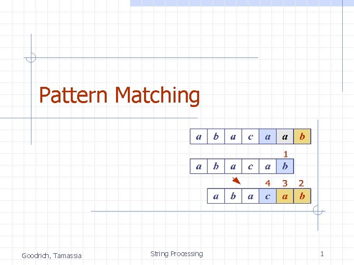
Pattern Matching Goodrich, Tamassia String Processing 1

Strings (§ 11. 1) Let P be a string of size m A string is a sequence of characters Examples of strings: n n n Java program HTML document DNA sequence Digitized image n An alphabet S is the set of possible characters for a family of strings Example of alphabets: n n ASCII Unicode {0, 1} {A, C, G, T} n Given strings T (text) and P (pattern), the pattern matching problem consists of finding a substring of T equal to P Applications: n n n Goodrich, Tamassia A substring P[i. . j] of P is the subsequence of P consisting of the characters with ranks between i and j A prefix of P is a substring of the type P[0. . i] A suffix of P is a substring of the type P[i. . m - 1] String Processing Text editors Search engines Biological research 2

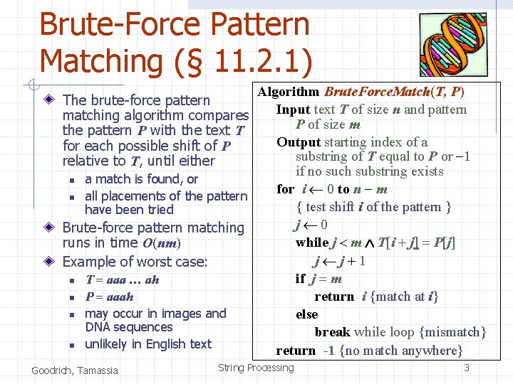
Brute-Force Pattern Matching (§ 11. 2. 1) Algorithm Brute. Force. Match(T, P) Input text T of size n and pattern P of size m Output starting index of a substring of T equal to P or -1 if no such substring exists n a match is found, or for i 0 to n - m n all placements of the pattern { test shift i of the pattern } have been tried j 0 Brute-force pattern matching while j < m T[i + j] = P[j] runs in time O(nm) j j+1 Example of worst case: if j = m n T = aaa … ah n P = aaah return i {match at i} n may occur in images and else DNA sequences break while loop {mismatch} n unlikely in English text return -1 {no match anywhere} The brute-force pattern matching algorithm compares the pattern P with the text T for each possible shift of P relative to T, until either Goodrich, Tamassia String Processing 3

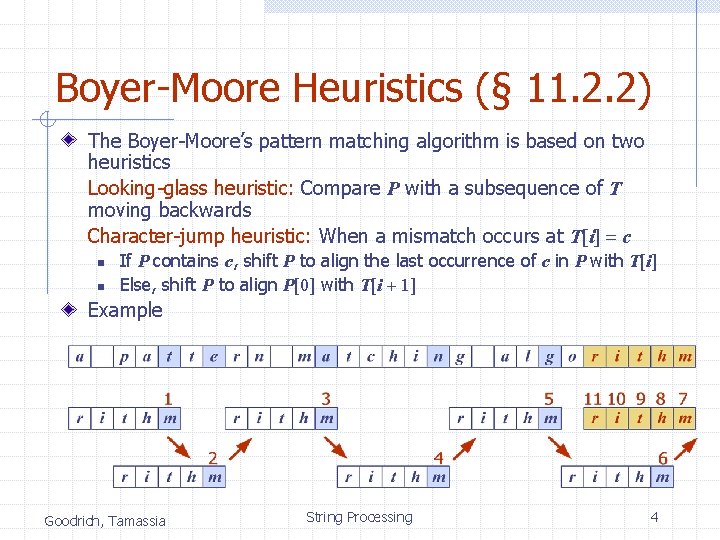
Boyer-Moore Heuristics (§ 11. 2. 2) The Boyer-Moore’s pattern matching algorithm is based on two heuristics Looking-glass heuristic: Compare P with a subsequence of T moving backwards Character-jump heuristic: When a mismatch occurs at T[i] = c n n If P contains c, shift P to align the last occurrence of c in P with T[i] Else, shift P to align P[0] with T[i + 1] Example Goodrich, Tamassia String Processing 4

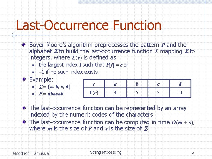
Last-Occurrence Function Boyer-Moore’s algorithm preprocesses the pattern P and the alphabet S to build the last-occurrence function L mapping S to integers, where L(c) is defined as n n the largest index i such that P[i] = c or -1 if no such index exists Example: n S = {a, b, c, d} n P = abacab c a b c d L(c) 4 5 3 -1 The last-occurrence function can be represented by an array indexed by the numeric codes of the characters The last-occurrence function can be computed in time O(m + s), where m is the size of P and s is the size of S Goodrich, Tamassia String Processing 5

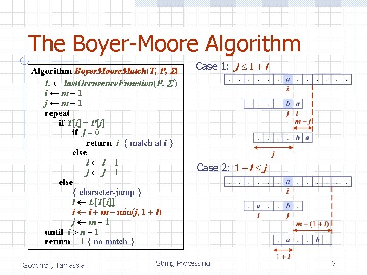
The Boyer-Moore Algorithm Boyer. Moore. Match(T, P, S) L last. Occurence. Function(P, S ) i m-1 j m-1 repeat if T[i] = P[j] if j = 0 return i { match at i } else i i-1 j j-1 else { character-jump } l L[T[i]] i i + m – min(j, 1 + l) j m-1 until i > n - 1 return -1 { no match } Goodrich, Tamassia Case 1: j 1 + l Case 2: 1 + l j String Processing 6

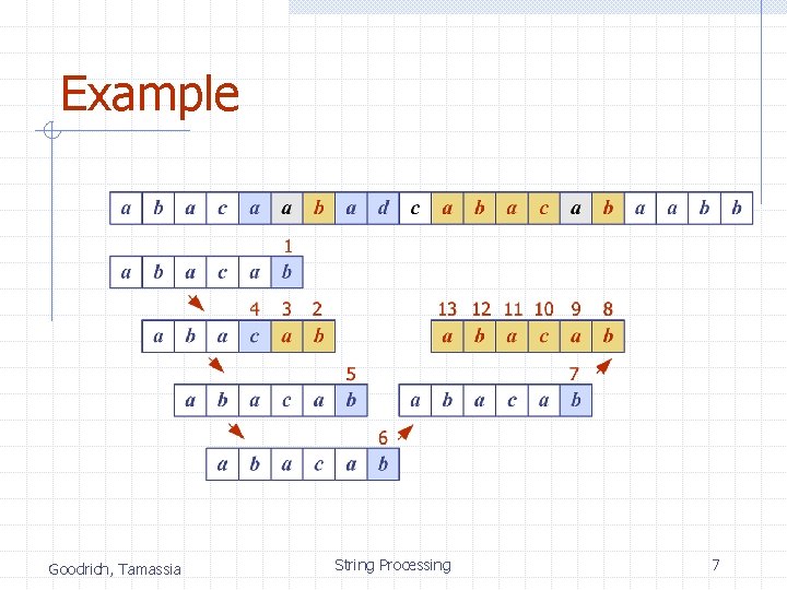
Example Goodrich, Tamassia String Processing 7

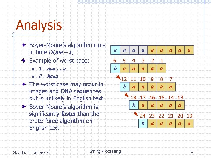
Analysis Boyer-Moore’s algorithm runs in time O(nm + s) Example of worst case: n n T = aaa … a P = baaa The worst case may occur in images and DNA sequences but is unlikely in English text Boyer-Moore’s algorithm is significantly faster than the brute-force algorithm on English text Goodrich, Tamassia String Processing 8

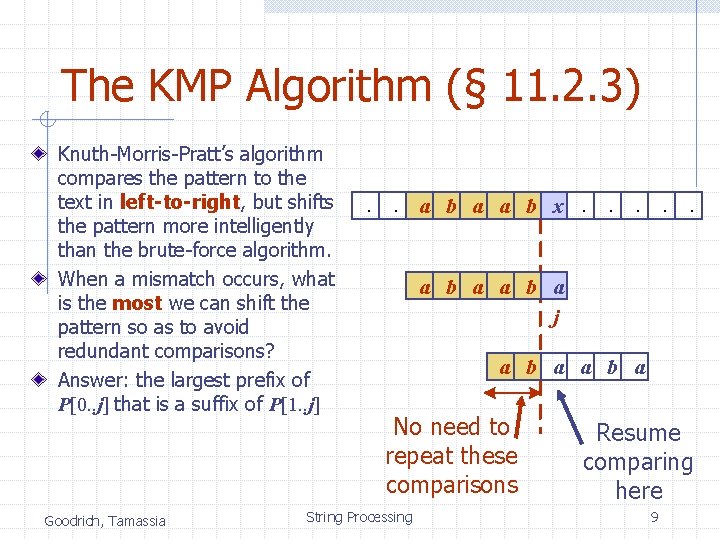
The KMP Algorithm (§ 11. 2. 3) Knuth-Morris-Pratt’s algorithm compares the pattern to the text in left-to-right, but shifts the pattern more intelligently than the brute-force algorithm. When a mismatch occurs, what is the most we can shift the pattern so as to avoid redundant comparisons? Answer: the largest prefix of P[0. . j] that is a suffix of P[1. . j] Goodrich, Tamassia . . a b a a b x. . . a b a j a b a No need to repeat these comparisons String Processing Resume comparing here 9

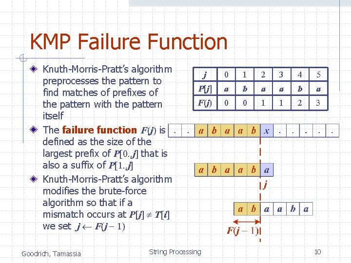
KMP Failure Function Knuth-Morris-Pratt’s algorithm preprocesses the pattern to find matches of prefixes of the pattern with the pattern itself The failure function F(j) is defined as the size of the largest prefix of P[0. . j] that is also a suffix of P[1. . j] Knuth-Morris-Pratt’s algorithm modifies the brute-force algorithm so that if a mismatch occurs at P[j] T[i] we set j F(j - 1) Goodrich, Tamassia j 0 1 2 3 4 5 P[j] a b a F(j) 0 0 1 1 2 3 String Processing 10

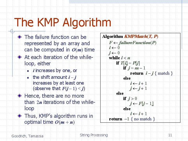
The KMP Algorithm The failure function can be represented by an array and can be computed in O(m) time At each iteration of the whileloop, either n n i increases by one, or the shift amount i - j increases by at least one (observe that F(j - 1) < j) Hence, there are no more than 2 n iterations of the whileloop Thus, KMP’s algorithm runs in optimal time O(m + n) Goodrich, Tamassia Algorithm KMPMatch(T, P) F failure. Function(P) i 0 j 0 while i < n if T[i] = P[j] if j = m - 1 return i - j { match } else i i+1 j j+1 else if j > 0 j F[j - 1] else i i+1 return -1 { no match } String Processing 11

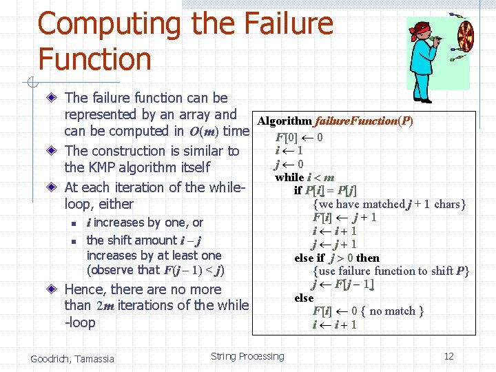
Computing the Failure Function The failure function can be represented by an array and Algorithm failure. Function(P) can be computed in O(m) time F[0] 0 i 1 The construction is similar to j 0 the KMP algorithm itself while i < m At each iteration of the whileif P[i] = P[j] {we have matched j + 1 chars} loop, either n n i increases by one, or the shift amount i - j increases by at least one (observe that F(j - 1) < j) Hence, there are no more than 2 m iterations of the while -loop Goodrich, Tamassia String Processing F[i] j + 1 i i+1 j j+1 else if j > 0 then {use failure function to shift P} j F[j - 1] else F[i] 0 { no match } i i+1 12
![Example j 0 1 2 3 4 5 Pj a b a c a Example j 0 1 2 3 4 5 P[j] a b a c a](https://slidetodoc.com/presentation_image_h2/10445d17398c70db55699f049cf73a04/image-13.jpg)
Example j 0 1 2 3 4 5 P[j] a b a c a b F(j) 0 0 1 2 Goodrich, Tamassia String Processing 13

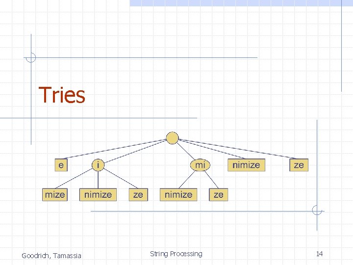
Tries Goodrich, Tamassia String Processing 14

Preprocessing Strings Preprocessing the pattern speeds up pattern matching queries n After preprocessing the pattern, KMP’s algorithm performs pattern matching in time proportional to the text size If the text is large, immutable and searched for often (e. g. , works by Shakespeare), we may want to preprocess the text instead of the pattern A trie is a compact data structure for representing a set of strings, such as all the words in a text n A tries supports pattern matching queries in time proportional to the pattern size Goodrich, Tamassia String Processing 15

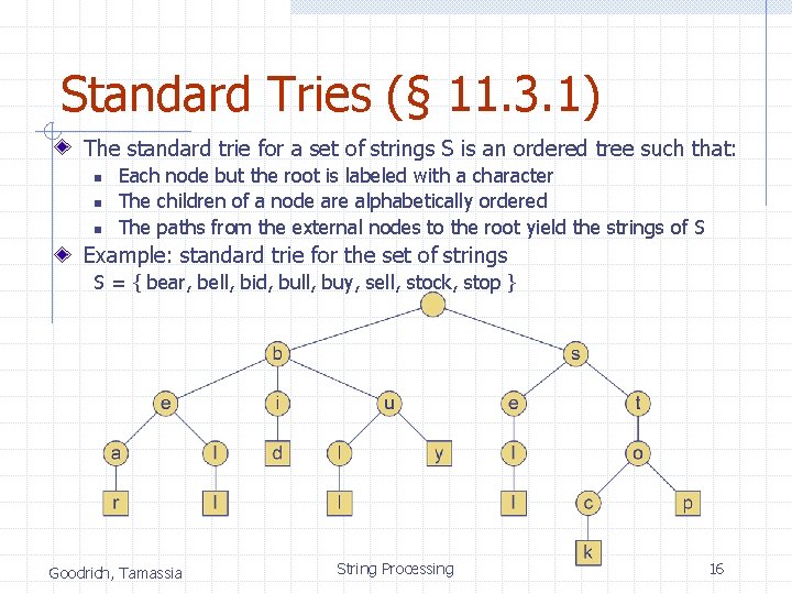
Standard Tries (§ 11. 3. 1) The standard trie for a set of strings S is an ordered tree such that: n n n Each node but the root is labeled with a character The children of a node are alphabetically ordered The paths from the external nodes to the root yield the strings of S Example: standard trie for the set of strings S = { bear, bell, bid, bull, buy, sell, stock, stop } Goodrich, Tamassia String Processing 16

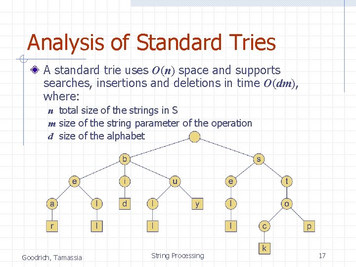
Analysis of Standard Tries A standard trie uses O(n) space and supports searches, insertions and deletions in time O(dm), where: n total size of the strings in S m size of the string parameter of the operation d size of the alphabet Goodrich, Tamassia String Processing 17

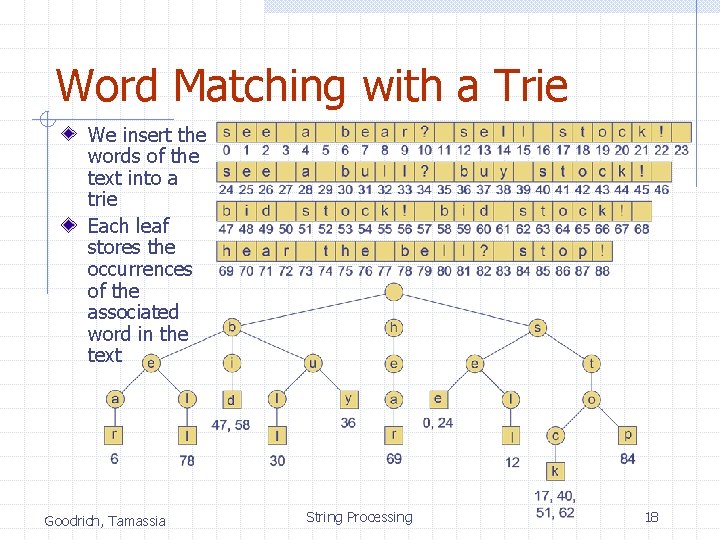
Word Matching with a Trie We insert the words of the text into a trie Each leaf stores the occurrences of the associated word in the text Goodrich, Tamassia String Processing 18

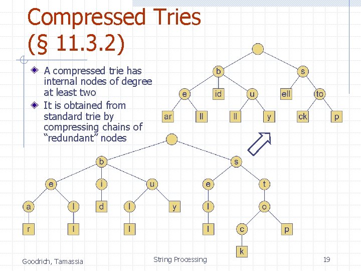
Compressed Tries (§ 11. 3. 2) A compressed trie has internal nodes of degree at least two It is obtained from standard trie by compressing chains of “redundant” nodes Goodrich, Tamassia String Processing 19

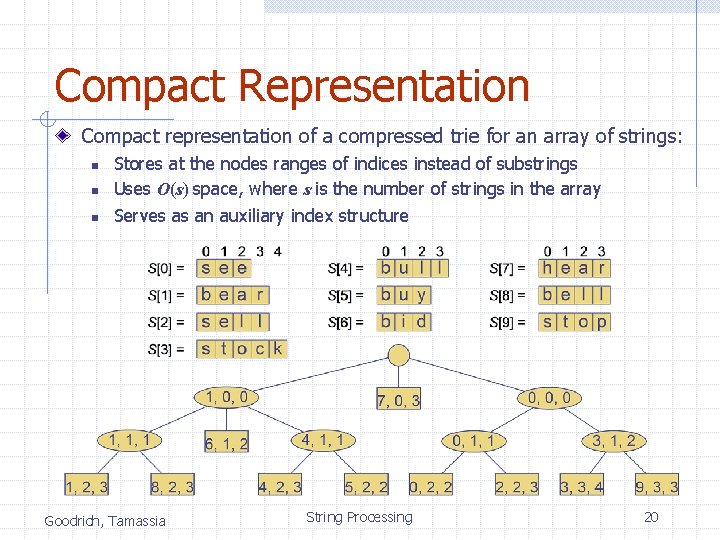
Compact Representation Compact representation of a compressed trie for an array of strings: n n n Stores at the nodes ranges of indices instead of substrings Uses O(s) space, where s is the number of strings in the array Serves as an auxiliary index structure Goodrich, Tamassia String Processing 20

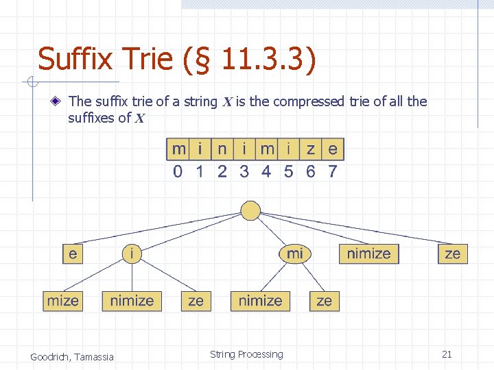
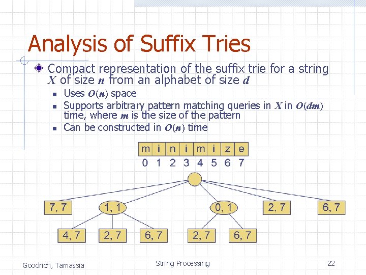
Suffix Trie (§ 11. 3. 3) The suffix trie of a string X is the compressed trie of all the suffixes of X Goodrich, Tamassia String Processing 21

Analysis of Suffix Tries Compact representation of the suffix trie for a string X of size n from an alphabet of size d n n n Uses O(n) space Supports arbitrary pattern matching queries in X in O(dm) time, where m is the size of the pattern Can be constructed in O(n) time Goodrich, Tamassia String Processing 22