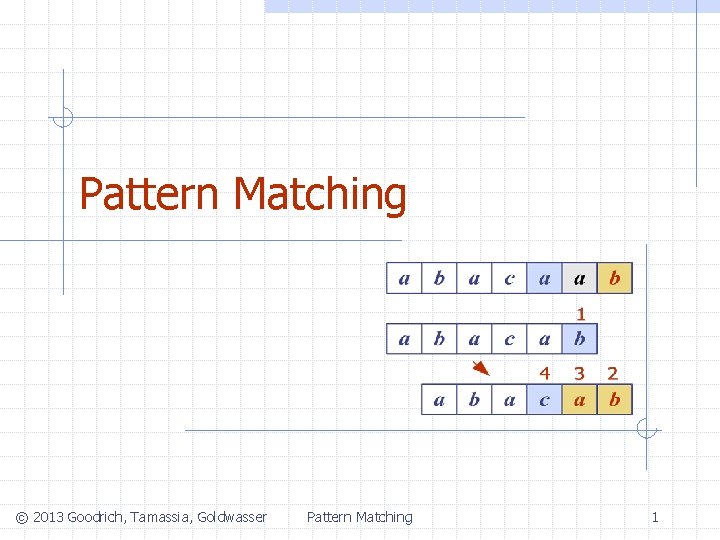
Pattern Matching 2013 Goodrich Tamassia Goldwasser Pattern Matching

Pattern Matching © 2013 Goodrich, Tamassia, Goldwasser Pattern Matching 1

Strings Let P be a string of size m A string is a sequence of characters Examples of strings: n n n Python program HTML document DNA sequence Digitized image n An alphabet S is the set of possible characters for a family of strings Example of alphabets: n n ASCII Unicode {0, 1} {A, C, G, T} n Given strings T (text) and P (pattern), the pattern matching problem consists of finding a substring of T equal to P Applications: n n n © 2013 Goodrich, Tamassia, Goldwasser A substring P[i. . j] of P is the subsequence of P consisting of the characters with ranks between i and j A prefix of P is a substring of the type P[0. . i] A suffix of P is a substring of the type P[i. . m - 1] Pattern Matching Text editors Search engines Biological research 2

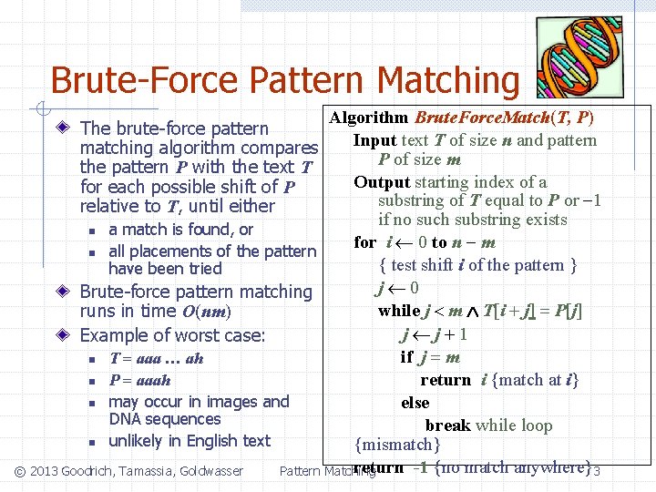
Brute-Force Pattern Matching Algorithm Brute. Force. Match(T, P) Input text T of size n and pattern P of size m Output starting index of a substring of T equal to P or -1 if no such substring exists n a match is found, or for i 0 to n - m n all placements of the pattern { test shift i of the pattern } have been tried j 0 Brute-force pattern matching while j < m T[i + j] = P[j] runs in time O(nm) j j+1 Example of worst case: if j = m n T = aaa … ah n P = aaah return i {match at i} n may occur in images and else DNA sequences break while loop n unlikely in English text {mismatch} return -1 {no match anywhere}3 Pattern Matching © 2013 Goodrich, Tamassia, Goldwasser The brute-force pattern matching algorithm compares the pattern P with the text T for each possible shift of P relative to T, until either

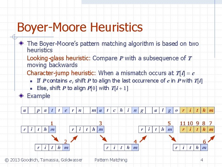
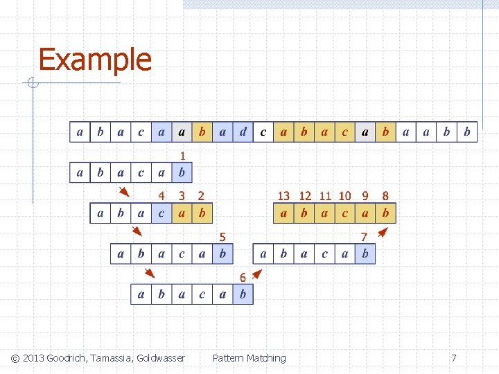
Boyer-Moore Heuristics The Boyer-Moore’s pattern matching algorithm is based on two heuristics Looking-glass heuristic: Compare P with a subsequence of T moving backwards Character-jump heuristic: When a mismatch occurs at T[i] = c n n If P contains c, shift P to align the last occurrence of c in P with T[i] Else, shift P to align P[0] with T[i + 1] Example © 2013 Goodrich, Tamassia, Goldwasser Pattern Matching 4

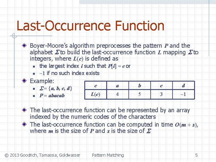
Last-Occurrence Function Boyer-Moore’s algorithm preprocesses the pattern P and the alphabet S to build the last-occurrence function L mapping S to integers, where L(c) is defined as n n the largest index i such that P[i] = c or -1 if no such index exists Example: n S = {a, b, c, d} n P = abacab c a b c d L(c) 4 5 3 -1 The last-occurrence function can be represented by an array indexed by the numeric codes of the characters The last-occurrence function can be computed in time O(m + s), where m is the size of P and s is the size of S © 2013 Goodrich, Tamassia, Goldwasser Pattern Matching 5

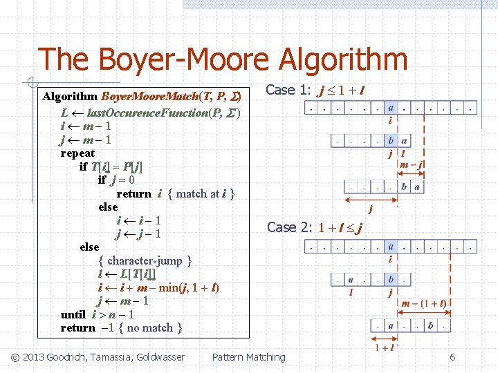
The Boyer-Moore Algorithm Boyer. Moore. Match(T, P, S) L last. Occurence. Function(P, S ) i m-1 j m-1 repeat if T[i] = P[j] if j = 0 return i { match at i } else i i-1 j j-1 else { character-jump } l L[T[i]] i i + m – min(j, 1 + l) j m-1 until i > n - 1 return -1 { no match } © 2013 Goodrich, Tamassia, Goldwasser Case 1: j 1 + l Case 2: 1 + l j Pattern Matching 6

Example © 2013 Goodrich, Tamassia, Goldwasser Pattern Matching 7

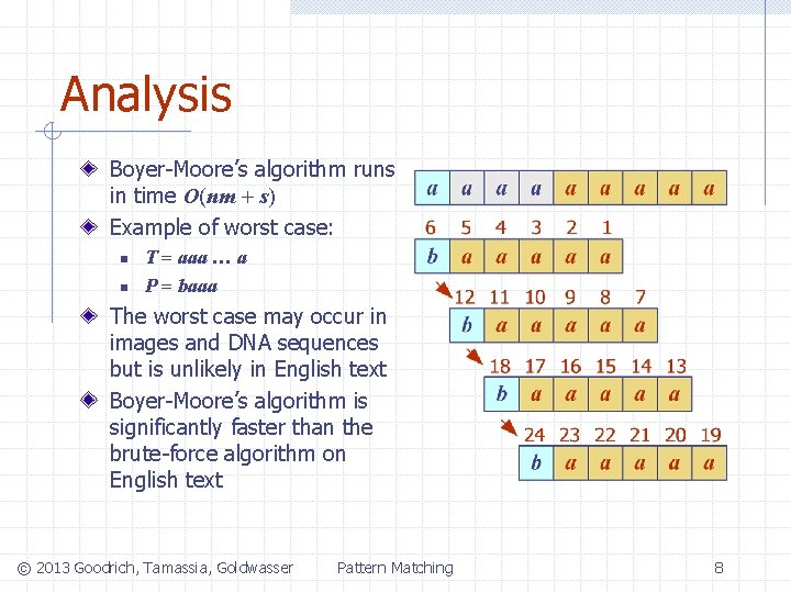
Analysis Boyer-Moore’s algorithm runs in time O(nm + s) Example of worst case: n n T = aaa … a P = baaa The worst case may occur in images and DNA sequences but is unlikely in English text Boyer-Moore’s algorithm is significantly faster than the brute-force algorithm on English text © 2013 Goodrich, Tamassia, Goldwasser Pattern Matching 8

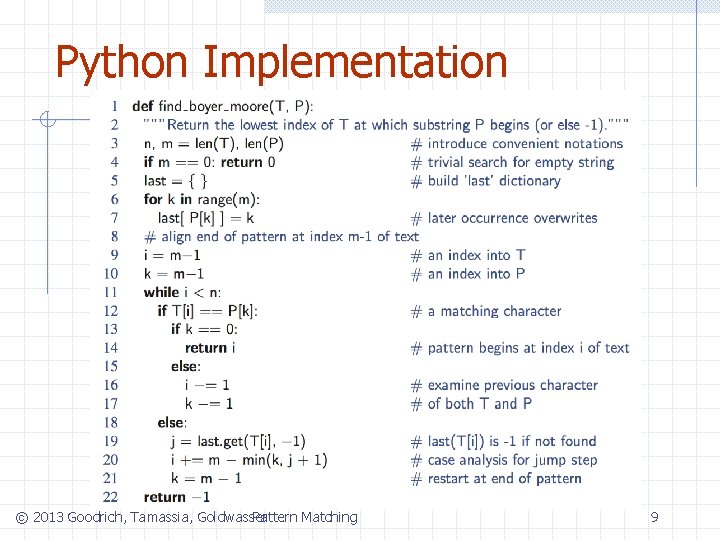
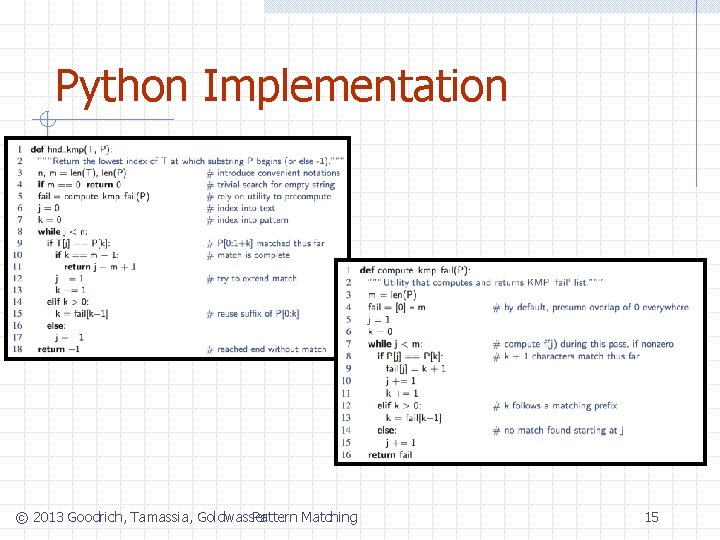
Python Implementation Pattern Matching © 2013 Goodrich, Tamassia, Goldwasser 9

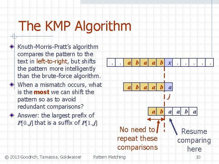
The KMP Algorithm Knuth-Morris-Pratt’s algorithm compares the pattern to the text in left-to-right, but shifts the pattern more intelligently than the brute-force algorithm. When a mismatch occurs, what is the most we can shift the pattern so as to avoid redundant comparisons? Answer: the largest prefix of P[0. . j] that is a suffix of P[1. . j] © 2013 Goodrich, Tamassia, Goldwasser . . a b a a b x. . . a b a j a b a No need to repeat these comparisons Pattern Matching Resume comparing here 10

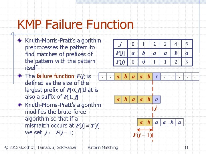
KMP Failure Function Knuth-Morris-Pratt’s algorithm preprocesses the pattern to find matches of prefixes of the pattern with the pattern itself The failure function F(j) is defined as the size of the largest prefix of P[0. . j] that is also a suffix of P[1. . j] Knuth-Morris-Pratt’s algorithm modifies the brute-force algorithm so that if a mismatch occurs at P[j] T[i] we set j F(j - 1) © 2013 Goodrich, Tamassia, Goldwasser j 0 1 2 3 4 5 P[j] a b a F(j) 0 0 1 1 2 3 Pattern Matching 11

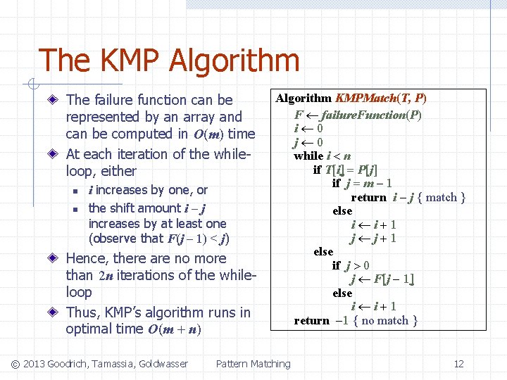
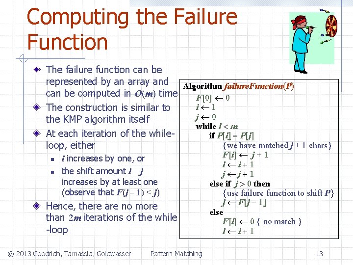
The KMP Algorithm The failure function can be represented by an array and can be computed in O(m) time At each iteration of the whileloop, either n n i increases by one, or the shift amount i - j increases by at least one (observe that F(j - 1) < j) Hence, there are no more than 2 n iterations of the whileloop Thus, KMP’s algorithm runs in optimal time O(m + n) © 2013 Goodrich, Tamassia, Goldwasser Algorithm KMPMatch(T, P) F failure. Function(P) i 0 j 0 while i < n if T[i] = P[j] if j = m - 1 return i - j { match } else i i+1 j j+1 else if j > 0 j F[j - 1] else i i+1 return -1 { no match } Pattern Matching 12

Computing the Failure Function The failure function can be represented by an array and Algorithm failure. Function(P) can be computed in O(m) time F[0] 0 i 1 The construction is similar to j 0 the KMP algorithm itself while i < m At each iteration of the whileif P[i] = P[j] {we have matched j + 1 chars} loop, either n n i increases by one, or the shift amount i - j increases by at least one (observe that F(j - 1) < j) Hence, there are no more than 2 m iterations of the while -loop © 2013 Goodrich, Tamassia, Goldwasser Pattern Matching F[i] j + 1 i i+1 j j+1 else if j > 0 then {use failure function to shift P} j F[j - 1] else F[i] 0 { no match } i i+1 13

Example j 0 1 2 3 4 5 P[j] a b a c a b F(j) 0 0 1 2 © 2013 Goodrich, Tamassia, Goldwasser Pattern Matching 14

Python Implementation Pattern Matching © 2013 Goodrich, Tamassia, Goldwasser 15