Past and Future Climate Simulation Lecture 3 GCMs

Past and Future Climate Simulation Lecture 3 – GCMs: parameterisations Ø (1) From last time – discretising the advection equation Ø (2) Parameterisations: clouds/precip, land surface, dust, the oceans. Ø (3) Implementation: boundary conditions, initial conditions. Ø (4) Model output and model-data comparison Ø (5) Experimental Design Ø (6) Model tuning

Example of numerics – atmospheric tracer 2 main parts to atmospheric GCM: 1) Adiabatic (no heat exchanged) – e. g. advection, surface friction. 2) Diabatic (heat exchanged) – e. g. radiation, boundary layer, clouds Adiabatic advection of a tracer. E. g. a volcanic ash cloud moving around the equator, in a wind of constant speed, u: u 180 W 180 E

name A B C D E F G H I J longitude 0 36 E 72 E 108 E 144 E 180 E 216 E 252 E 288 E 324 E Initial Concentration 0 1 0 0 0 0 U=0. 1 Excel demonstration A 0=0, B 0=1, C 0=0, …… A 1=0, B 1=B 0 -0. 1, C 1=C 0+0. 1, D 1=0, …… name A B C D E F G H I J longitude 0 36 E 72 E 108 E 144 E 180 E 216 E 252 E 288 E 324 E Initial Concentration 0 1 0 0 0 0 Concentration after 1 timestep 0 0. 9 0. 1 0 0 0 0 Concentration after 2 timesteps 0 0. 81 0. 18 0. 01 0 0 0

(2) Parameterisations 2 main parts to atmospheric GCM: 1) Adiabatic (momentum equation, last lecture) 2) Diabatic (heat exchanged) – e. g. convection, radiation (including clouds, greenhouse gases, aerosols), precipitation, surface energy balance. All parameterisations. e. g. precipitation: e. g. convection: If (relative humidity > 85%) then If (temperature gradient > 10 o. C/km) then precipitation = (relative humidity 85%)*constant relative humidity = 85% clouds = 1 temperature gradient = 10 o. C/km precipitation

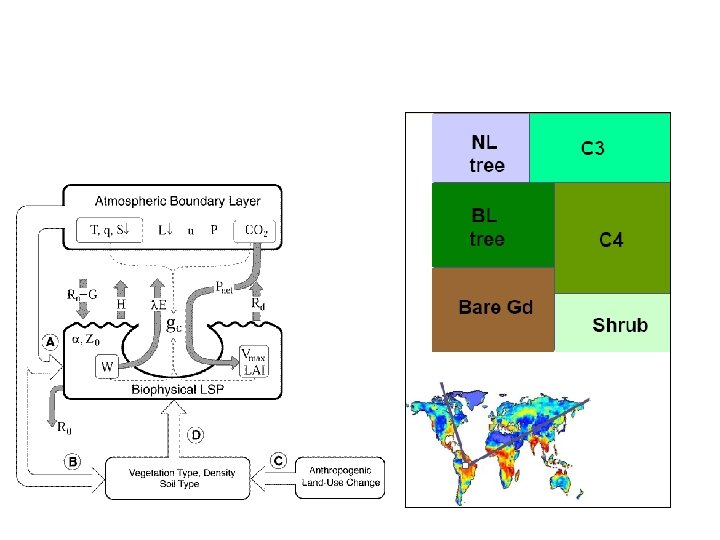
e. g. land surface and turbulence:

e. g. aerosols (here, dust): (1) Potential dust source regions

(2) Wind speed…. ~ u 3 with a threshold….

(3) Gusts…. convection (4) Soil moisture…. (5) Wet deposition…

(6) Dry deposition… (7) Evaluation

e. g. oceans: Simulate just the uppermost approx 50 m of the ocean (homogeneous slab of water). Typically, atmosphere calculates the surface energy fluxes for each gridbox (net-solar, net-infrared, sensible, latent heats). The sum will not be zero; this is the net energy flux at the surface. If it is positive, the ocean absorbs this and warms up appropriately. If it is negative the ocean will cool down. 1) 2) Need to parameterise ocean heat transport! Therefore no good for time periods/climates very different from modern.

(3) Configuring Models – boundary conditions/initial conditions Boundary Conditions: Prescribed (by the user) fields. e. g. landsea mask. The model can not change these. May be time-varying (e. g. SST). Initial Conditions: Fields used for initialising the model. After first timestep, model calculates. e. g. surface temperature

Boundary conditions Land-sea mask

Orography

Sub-gridscale orography

Bathymetry

Surface albedo (for models not predicting vegetation)

Sea surface temperatures (for models without an ocean)

Incoming solar radiation

Greenhouse gases, aerosols

Initial conditions Surface Temperature Cloud cover Pressure in mid-atmosphere Soil moisture + for ocean: temp, salinity, u, v, seaice

(4) Model output and model-data comparison

Produce a ‘climatology’

Model-data comparison…

Surface Temperature: observations Surface Temperature: Had. CM 3 How good are GCMs? (1) temperature

Precipitation: observations Seaice: observations vs models Precipitation: Had. CM 3 How good are GCMs? (2) Precip and seaice

How good are GCMs? (3) El Nino

(5) Experimental Design Key concept: Testing hypotheses. Typically, a ‘control’ + a number of ‘sensitivity studies’ • Modify a boundary condition… “If everyone painted their roofs white, could this mitigate against global warming? ” • Modify an internal parameter… “Can the fact that all models predict too-cold poles in deep-time palaeoclimates be due to the lack of anthropogenic aerosols? ” • Modify an initial condition… “Was the Sahara bistable in the mid-Holcoene, 6, 000 years ago? ” • Change a parameterisation… “Does poor representation of clouds in models result in poor ENSO simulation? ” • Change the whole model… “Which is the best model to use for future climate prediction? ”

(6) Model Tuning We know that internal model parameters affect the control climate produced by a model…often these are not well constrained by data. Therefore we can legitimately ‘tune’ the model towards observations of modern climate by ‘tweaking’ these parameters… For a small number of parameters, we can cover ‘parameter space’ well…but…. N=Ax , where N is number of simulations, A is how well we sample the parameter space, and x is the number of parameters…. soon become unmanageable. So, various approaches, including random sampling…. .

And ‘latin hypercube’ sampling…. . Skill score generated, and then experiments ranked. . .

Tuned model outperforms original model…. . observations tuned model original model