Partitioning 1 Partitioning Decomposition of a complex system

Partitioning 1

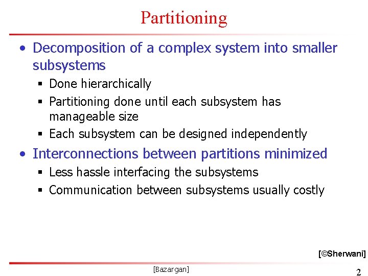
Partitioning • Decomposition of a complex system into smaller subsystems § Done hierarchically § Partitioning done until each subsystem has manageable size § Each subsystem can be designed independently • Interconnections between partitions minimized § Less hassle interfacing the subsystems § Communication between subsystems usually costly [©Sherwani] [Bazargan] 2

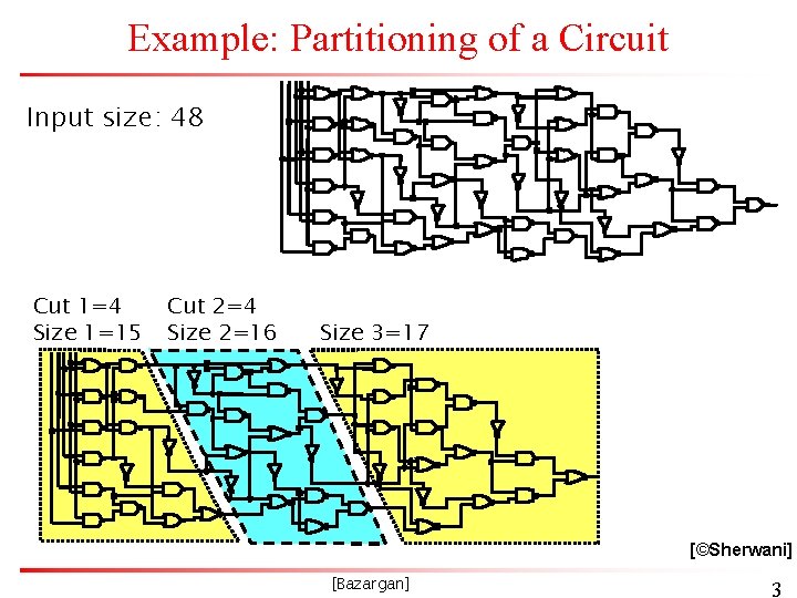
Example: Partitioning of a Circuit Input size: 48 Cut 1=4 Size 1=15 Cut 2=4 Size 2=16 Size 3=17 [©Sherwani] [Bazargan] 3

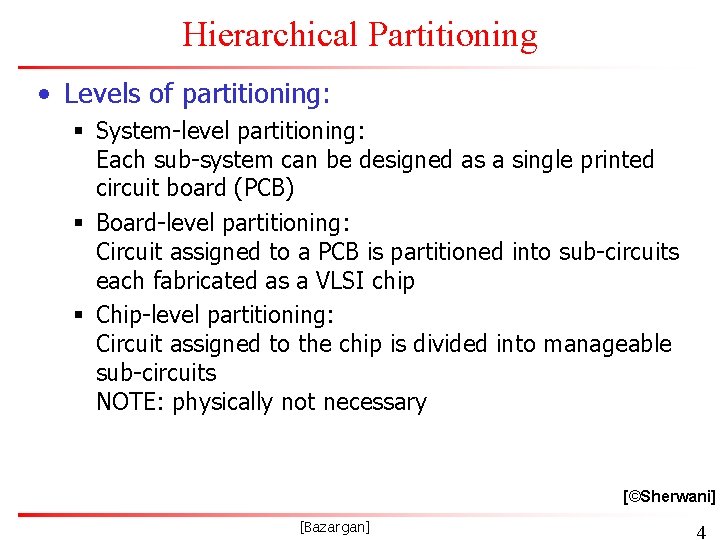
Hierarchical Partitioning • Levels of partitioning: § System-level partitioning: Each sub-system can be designed as a single printed circuit board (PCB) § Board-level partitioning: Circuit assigned to a PCB is partitioned into sub-circuits each fabricated as a VLSI chip § Chip-level partitioning: Circuit assigned to the chip is divided into manageable sub-circuits NOTE: physically not necessary [©Sherwani] [Bazargan] 4

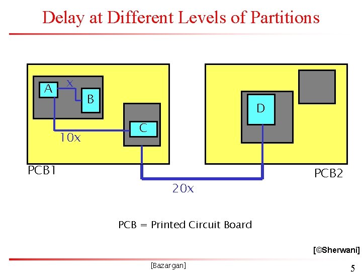
Delay at Different Levels of Partitions A x 10 x PCB 1 B D C 20 x PCB 2 PCB = Printed Circuit Board [©Sherwani] [Bazargan] 5

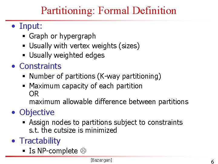
Partitioning: Formal Definition • Input: § Graph or hypergraph § Usually with vertex weights (sizes) § Usually weighted edges • Constraints § Number of partitions (K-way partitioning) § Maximum capacity of each partition OR maximum allowable difference between partitions • Objective § Assign nodes to partitions subject to constraints s. t. the cutsize is minimized • Tractability § Is NP-complete [Bazargan] 6

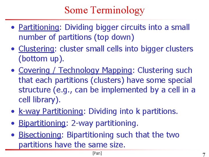
Some Terminology • Partitioning: Dividing bigger circuits into a small number of partitions (top down) • Clustering: cluster small cells into bigger clusters (bottom up). • Covering / Technology Mapping: Clustering such that each partitions (clusters) have some special structure (e. g. , can be implemented by a cell in a cell library). • k-way Partitioning: Dividing into k partitions. • Bipartitioning: 2 -way partitioning. • Bisectioning: Bipartitioning such that the two partitions have the same size. [Pan] 7

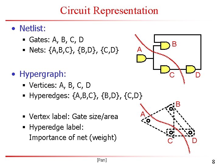
Circuit Representation • Netlist: § Gates: A, B, C, D § Nets: {A, B, C}, {B, D}, {C, D} A • Hypergraph: B C D § Vertices: A, B, C, D § Hyperedges: {A, B, C}, {B, D}, {C, D} B § Vertex label: Gate size/area § Hyperedge label: Importance of net (weight) [Pan] A C D 8

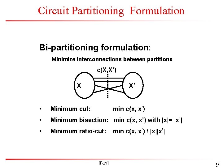
Circuit Partitioning Formulation Bi-partitioning formulation: Minimize interconnections between partitions c(X, X’) X X’ • Minimum cut: • Minimum bisection: min c(x, x’) with |x|= |x’| • Minimum ratio-cut: min c(x, x’) [Pan] min c(x, x’) / |x||x’| 9

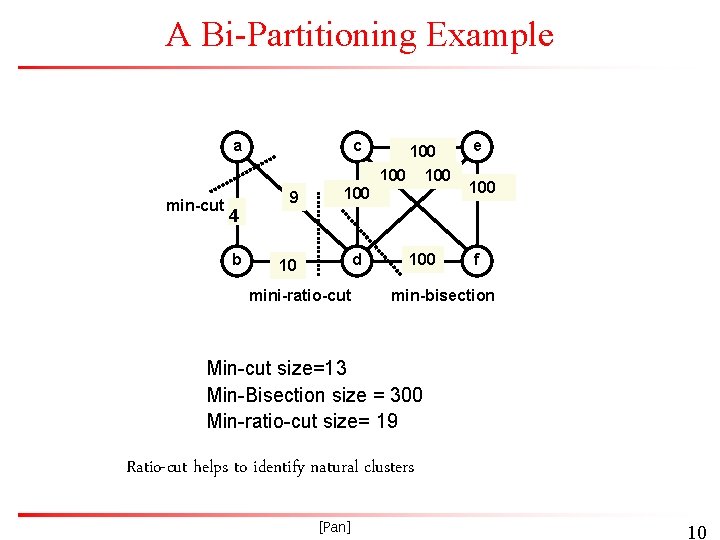
A Bi-Partitioning Example a min-cut 4 b c 9 100 100 d 10 mini-ratio-cut 100 e 100 f min-bisection Min-cut size=13 Min-Bisection size = 300 Min-ratio-cut size= 19 Ratio-cut helps to identify natural clusters [Pan] 10

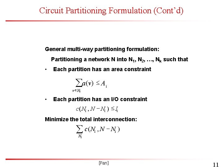
Circuit Partitioning Formulation (Cont’d) General multi-way partitioning formulation: Partitioning a network N into N 1, N 2, …, Nk such that • Each partition has an area constraint a(v) A v Ni • i Each partition has an I/O constraint c( Ni , N - Ni ) Ii Minimize the total interconnection: c( N , N - N ) i i Ni [Pan] 11

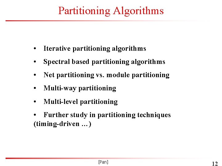
Partitioning Algorithms • Iterative partitioning algorithms • Spectral based partitioning algorithms • Net partitioning vs. module partitioning • Multi-way partitioning • Multi-level partitioning • Further study in partitioning techniques (timing-driven …) [Pan] 12

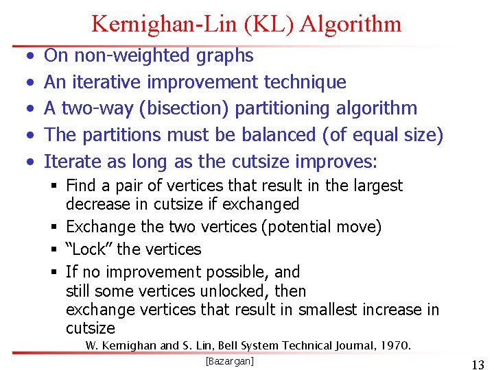
Kernighan-Lin (KL) Algorithm • • • On non-weighted graphs An iterative improvement technique A two-way (bisection) partitioning algorithm The partitions must be balanced (of equal size) Iterate as long as the cutsize improves: § Find a pair of vertices that result in the largest decrease in cutsize if exchanged § Exchange the two vertices (potential move) § “Lock” the vertices § If no improvement possible, and still some vertices unlocked, then exchange vertices that result in smallest increase in cutsize W. Kernighan and S. Lin, Bell System Technical Journal, 1970. [Bazargan] 13

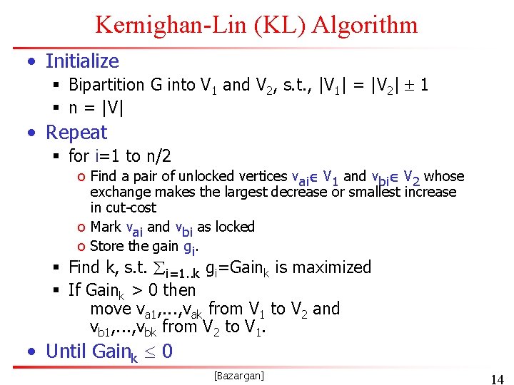
Kernighan-Lin (KL) Algorithm • Initialize § Bipartition G into V 1 and V 2, s. t. , |V 1| = |V 2| 1 § n = |V| • Repeat § for i=1 to n/2 o Find a pair of unlocked vertices vai V 1 and vbi V 2 whose exchange makes the largest decrease or smallest increase in cut-cost o Mark vai and vbi as locked o Store the gain gi. § Find k, s. t. i=1. . k gi=Gaink is maximized § If Gaink > 0 then move va 1, . . . , vak from V 1 to V 2 and vb 1, . . . , vbk from V 2 to V 1. • Until Gaink 0 [Bazargan] 14

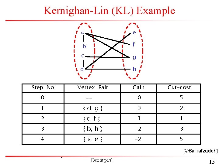
Kernighan-Lin (KL) Example Step No. 0 a e b f c g d h Vertex Pair -- Gain Cut-cost 0 5 1 { d, g } 3 2 2 { c, f } 1 1 3 { b, h } -2 3 4 { a, e } -2 5 [©Sarrafzadeh] [Bazargan] 15

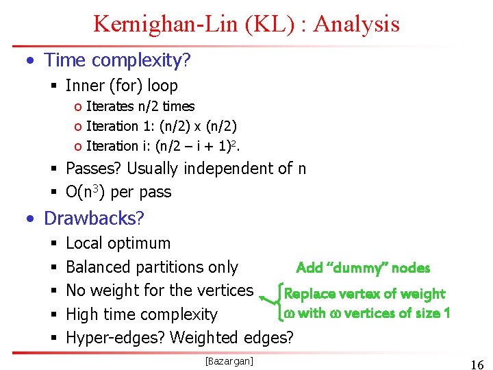
Kernighan-Lin (KL) : Analysis • Time complexity? § Inner (for) loop o Iterates n/2 times o Iteration 1: (n/2) x (n/2) o Iteration i: (n/2 – i + 1)2. § Passes? Usually independent of n § O(n 3) per pass • Drawbacks? § § § Local optimum Balanced partitions only Add “dummy” nodes No weight for the vertices Replace vertex of weight w with w vertices of size 1 High time complexity Hyper-edges? Weighted edges? [Bazargan] 16

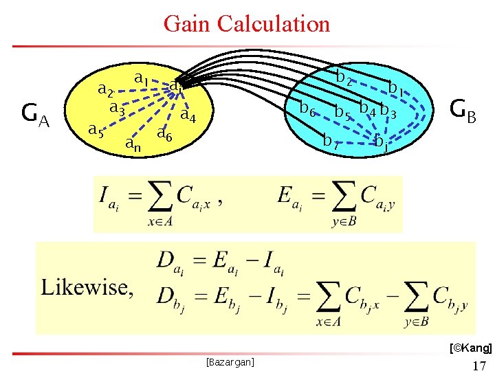
Gain Calculation GA a 2 a 3 a 5 a 1 an b 2 ai a 6 b 6 a 4 b 1 b 5 b 4 b 3 b 7 bj GB External cost Internal cost [©Kang] [Bazargan] 17

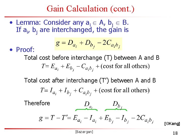
Gain Calculation (cont. ) • Lemma: Consider any ai A, bj B. If ai, bj are interchanged, the gain is • Proof: Total cost before interchange (T) between A and B Total cost after interchange (T’) between A and B Therefore [©Kang] [Bazargan] 18

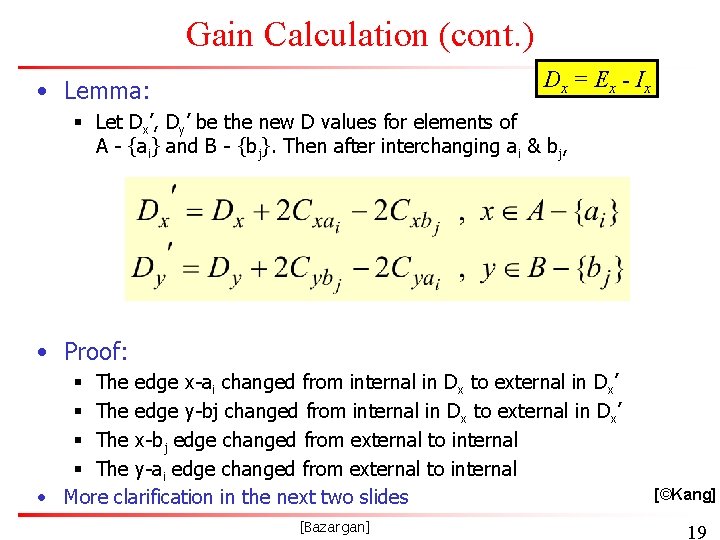
Gain Calculation (cont. ) D x = E x - Ix • Lemma: § Let Dx’, Dy’ be the new D values for elements of A - {ai} and B - {bj}. Then after interchanging ai & bj, • Proof: § The edge x-ai changed from internal in Dx to external in Dx’ § The edge y-bj changed from internal in Dx to external in Dx’ § The x-bj edge changed from external to internal § The y-ai edge changed from external to internal • More clarification in the next two slides [Bazargan] [©Kang] 19

Clarification of the Lemma b a bj x ai [Bazargan] 20

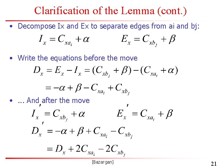
Clarification of the Lemma (cont. ) • Decompose Ix and Ex to separate edges from ai and bj: • Write the equations before the move • . . . And after the move [Bazargan] 21

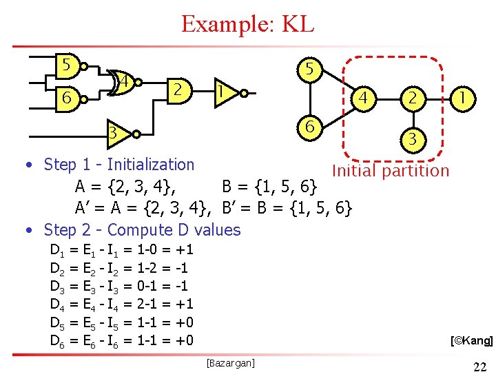
Example: KL 5 4 6 2 1 5 4 6 3 2 1 3 • Step 1 - Initialization Initial partition A = {2, 3, 4}, B = {1, 5, 6} A’ = A = {2, 3, 4}, B’ = B = {1, 5, 6} • Step 2 - Compute D values D 1 D 2 D 3 D 4 D 5 D 6 = = = E 1 E 2 E 3 E 4 E 5 E 6 - I 1 I 2 I 3 I 4 I 5 I 6 = = = 1 -0 1 -2 0 -1 2 -1 1 -1 = = = +1 -1 -1 +1 +0 +0 [©Kang] [Bazargan] 22

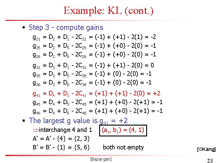
Example: KL (cont. ) § Step 3 - compute gains g 21 = D 2 + D 1 - 2 C 21 = (-1) + (+1) - 2(1) = -2 g 25 = D 2 + D 5 - 2 C 25 = (-1) + (+0) - 2(0) = -1 g 26 = D 2 + D 6 - 2 C 26 = (-1) + (+0) - 2(0) = -1 g 31 = D 3 + D 1 - 2 C 31 = (-1) + (+1) - 2(0) = 0 g 35 = D 3 + D 5 - 2 C 35 = (-1) + (0) - 2(0) = -1 g 36 = D 3 + D 6 - 2 C 36 = (-1) + (0) - 2(0) = -1 g 41 = D 4 + D 1 - 2 C 41 = (+1) + (+1) - 2(0) = +2 g 45 = D 4 + D 5 - 2 C 45 = (+1) + (+0) - 2(+1) = -1 g 46 = D 4 + D 6 - 2 C 46 = (+1) + (+0) - 2(+1) = -1 § The largest g value is g 41 = +2 Þinterchange 4 and 1 A’ = A’ - {4} = {2, 3} B’ = B’ - {1} = {5, 6} (a 1, b 1) = (4, 1) both not empty [Bazargan] [©Kang] 23

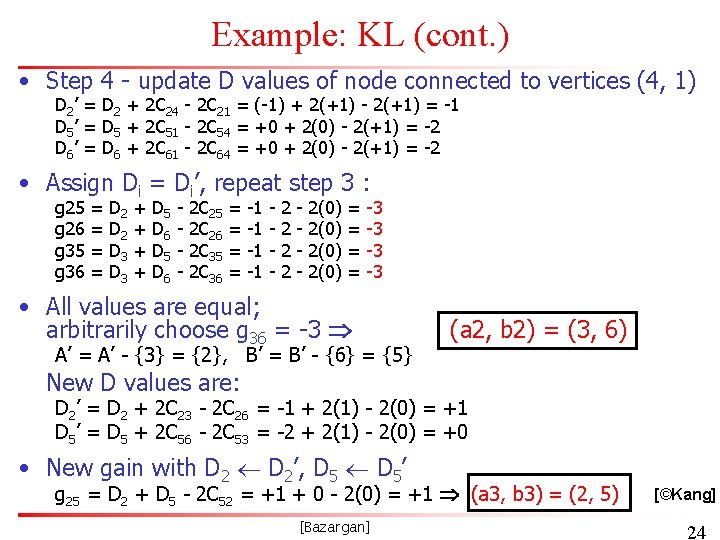
Example: KL (cont. ) • Step 4 - update D values of node connected to vertices (4, 1) D 2’ = D 2 + 2 C 24 - 2 C 21 = (-1) + 2(+1) - 2(+1) = -1 D 5’ = D 5 + 2 C 51 - 2 C 54 = +0 + 2(0) - 2(+1) = -2 D 6’ = D 6 + 2 C 61 - 2 C 64 = +0 + 2(0) - 2(+1) = -2 • Assign Di = Di’, repeat step 3 : g 25 g 26 g 35 g 36 = = D 2 D 3 + + D 5 D 6 - 2 C 25 2 C 26 2 C 35 2 C 36 = = -1 -1 - 2 2 - 2(0) = = -3 -3 • All values are equal; arbitrarily choose g 36 = -3 A’ = A’ - {3} = {2}, B’ = B’ - {6} = {5} (a 2, b 2) = (3, 6) New D values are: D 2’ = D 2 + 2 C 23 - 2 C 26 = -1 + 2(1) - 2(0) = +1 D 5’ = D 5 + 2 C 56 - 2 C 53 = -2 + 2(1) - 2(0) = +0 • New gain with D 2’, D 5’ g 25 = D 2 + D 5 - 2 C 52 = +1 + 0 - 2(0) = +1 (a 3, b 3) = (2, 5) [Bazargan] [©Kang] 24

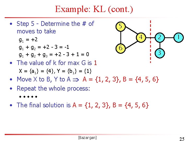
Example: KL (cont. ) • Step 5 - Determine the # of moves to take g 1 = +2 g 1 + g 2 = +2 - 3 = -1 g 1 + g 2 + g 3 = +2 - 3 + 1 = 0 5 4 6 2 1 3 • The value of k for max G is 1 X = {a 1} = {4}, Y = {b 1} = {1} • Move X to B, Y to A A = {1, 2, 3}, B = {4, 5, 6} • Repeat the whole process: • • • • The final solution is A = {1, 2, 3}, B = {4, 5, 6} [Bazargan] 25

Fiduccia-Mattheyses (FM) Algorithm • Modified version of KL • A single vertex is moved across the cut in a single move § Unbalanced partitions • Vertices are weighted • Concept of cutsize extended to hypergraphs • Special data structure to improve time complexity to O(n 2) per pass § (Main feature) • Can be extended to multi-way partitioning C. M. Fiduccia and R. M. Mattheyses, 19 th DAC, 1982. [Bazargan] 26

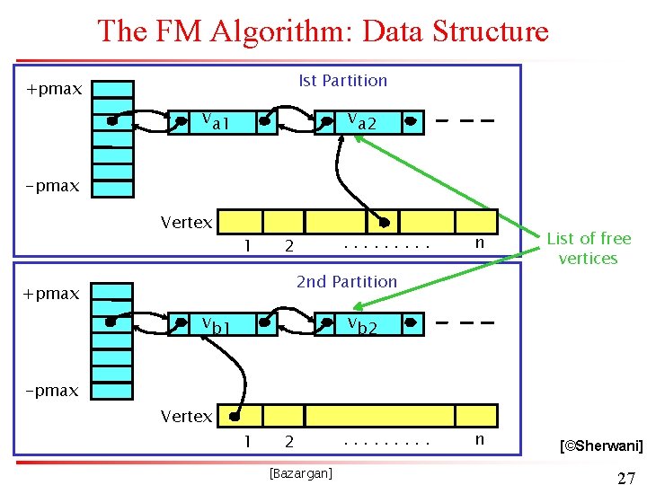
The FM Algorithm: Data Structure Ist Partition +pmax va 1 va 2 -pmax Vertex 1 . . 2 n 2 nd Partition +pmax vb 1 List of free vertices vb 2 -pmax Vertex 1 2 [Bazargan] . . n [©Sherwani] 27

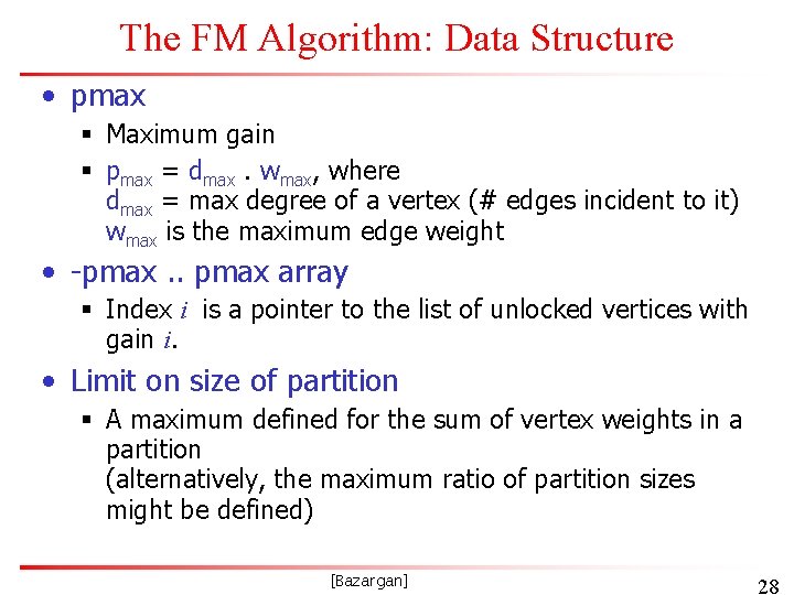
The FM Algorithm: Data Structure • pmax § Maximum gain § pmax = dmax. wmax, where dmax = max degree of a vertex (# edges incident to it) wmax is the maximum edge weight • -pmax. . pmax array § Index i is a pointer to the list of unlocked vertices with gain i. • Limit on size of partition § A maximum defined for the sum of vertex weights in a partition (alternatively, the maximum ratio of partition sizes might be defined) [Bazargan] 28

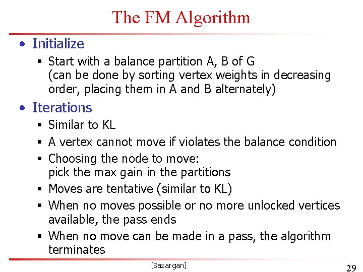
The FM Algorithm • Initialize § Start with a balance partition A, B of G (can be done by sorting vertex weights in decreasing order, placing them in A and B alternately) • Iterations § Similar to KL § A vertex cannot move if violates the balance condition § Choosing the node to move: pick the max gain in the partitions § Moves are tentative (similar to KL) § When no moves possible or no more unlocked vertices available, the pass ends § When no move can be made in a pass, the algorithm terminates [Bazargan] 29

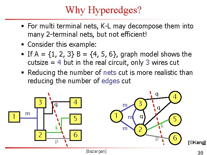
Why Hyperedges? § For multi terminal nets, K-L may decompose them into many 2 -terminal nets, but not efficient! § Consider this example: § If A = {1, 2, 3} B = {4, 5, 6}, graph model shows the cutsize = 4 but in the real circuit, only 3 wires cut § Reducing the number of nets cut is more realistic than reducing the number of edges cut 3 1 q m 2 k p q 4 3 m 1 5 m m 6 [Bazargan] 4 q q 2 k p 5 6 [©Kang] 30

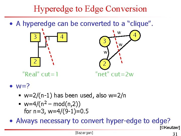
Hyperedge to Edge Conversion • A hyperedge can be converted to a “clique”. 3 1 w 4 3 4 w w 2 2 “Real” cut=1 “net” cut=2 w • w=? § w=2/(n-1) has been used, also w=2/n § w=4/(n 2 – mod(n, 2)) for n=3, w=4/(9 -1)=0. 5 • Always necessary to convert hyper-edge to edge? [©Keutzer] [Bazargan] 31

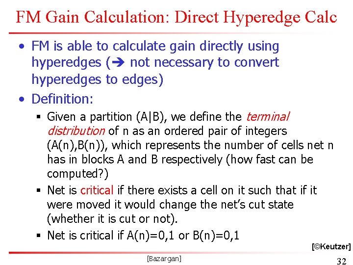
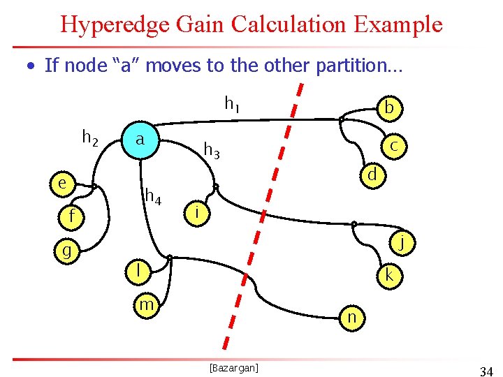
FM Gain Calculation: Direct Hyperedge Calc • FM is able to calculate gain directly using hyperedges ( not necessary to convert hyperedges to edges) • Definition: § Given a partition (A|B), we define the terminal distribution of n as an ordered pair of integers (A(n), B(n)), which represents the number of cells net n has in blocks A and B respectively (how fast can be computed? ) § Net is critical if there exists a cell on it such that if it were moved it would change the net’s cut state (whether it is cut or not). § Net is critical if A(n)=0, 1 or B(n)=0, 1 [©Keutzer] [Bazargan] 32

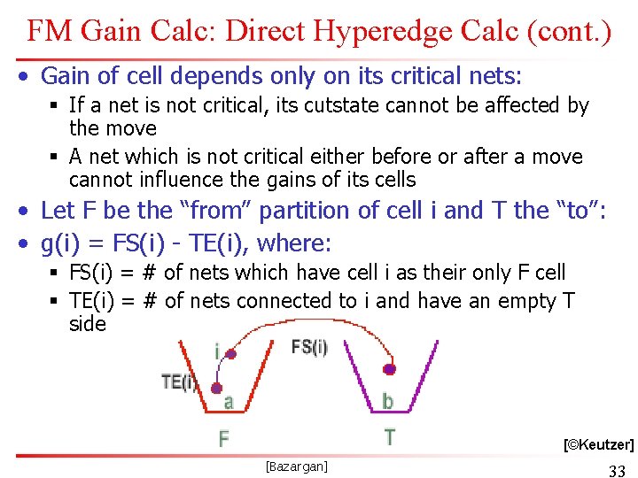
FM Gain Calc: Direct Hyperedge Calc (cont. ) • Gain of cell depends only on its critical nets: § If a net is not critical, its cutstate cannot be affected by the move § A net which is not critical either before or after a move cannot influence the gains of its cells • Let F be the “from” partition of cell i and T the “to”: • g(i) = FS(i) - TE(i), where: § FS(i) = # of nets which have cell i as their only F cell § TE(i) = # of nets connected to i and have an empty T side [©Keutzer] [Bazargan] 33

Hyperedge Gain Calculation Example • If node “a” moves to the other partition… h 1 h 2 a e h 4 f g b c h 3 d i j l k m n [Bazargan] 34

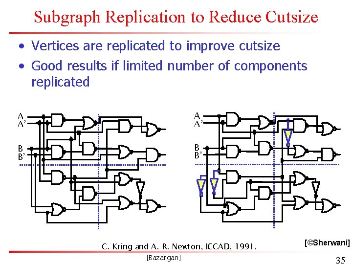
Subgraph Replication to Reduce Cutsize • Vertices are replicated to improve cutsize • Good results if limited number of components replicated A A’ B B’ C. Kring and A. R. Newton, ICCAD, 1991. [Bazargan] [©Sherwani] 35

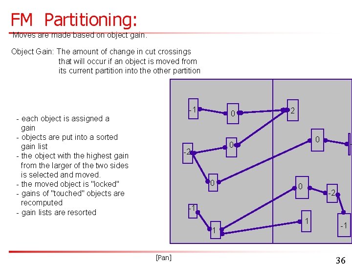
FM Partitioning: Moves are made based on object gain. Object Gain: The amount of change in cut crossings that will occur if an object is moved from its current partition into the other partition -1 - each object is assigned a gain - objects are put into a sorted gain list - the object with the highest gain from the larger of the two sides is selected and moved. - the moved object is "locked" - gains of "touched" objects are recomputed - gain lists are resorted 0 2 0 0 - -2 -1 1 1 [Pan] -1 36

FM Partitioning: -1 0 2 0 0 - -2 -1 1 1 [Pan] -1 37

-1 -2 -2 0 0 - -2 -1 1 1 [Pan] -1 38

-1 -2 -2 0 0 - -2 -1 1 [Pan] 1 -1 39

-1 -2 -2 0 -1 [Pan] 0 1 - -2 1 -1 40

-1 -2 -2 0 1 [Pan] -2 -1 -1 - -2 -1 41

-1 -2 -2 0 1 [Pan] - 0 -2 -1 -1 -2 -1 42

-1 -2 -2 -2 0 0 1 [Pan] -2 -1 -1 -2 -1 43

-1 -2 -2 0 -2 1 [Pan] -2 -1 -1 -2 -1 44

-1 -2 -2 0 -2 -2 1 -1 [Pan] -1 -2 -1 45

-1 -2 -2 0 -2 -2 1 -1 [Pan] -1 -2 -1 46

-1 -2 -2 0 -2 -1 -3 [Pan] -2 -1 47

-1 -2 -2 0 -1 -2 -2 -3 [Pan] -1 -2 -1 48

-1 -2 -2 0 -1 -2 -2 -3 [Pan] -1 -2 -1 49

-1 -2 -2 -3 [Pan] -1 -2 -1 50

Time Complexity of FM • For each pass, § Constant time to find the best vertex to move. § After each move, time to update gain buckets is proportional to degree of vertex moved. § Total time is O(p), where p is total number of pins • Number of passes is usually small. [Pan] 51

Extension by Krishnamurthy “An Improved Min-Cut Algorithm for Partitioning VLSI Networks”, IEEE Trans. Computer, 33(5): 438 -446, 1984. [Pan] 52

Tie-Breaking Strategy • For each vertex, instead of having a gain bucket, a gain vector is used. • Gain vector is a sequence of potential gain values corresponding to numbers of possible moves into the future. • Therefore, rth entry looks r moves ahead. • Time complexity is O(pr), where r is max # of lookahead moves stored in gain vector. • If ties still occur, some researchers observe that LIFO order improves solution quality. [Pan] 53

Ratio Cut Objective by Wei and Cheng “Towards Efficient Hierarchical Designs by Ratio Cut Partitioning”, ICCAD, pages 1: 298 -301, 1989. [Pan] 54

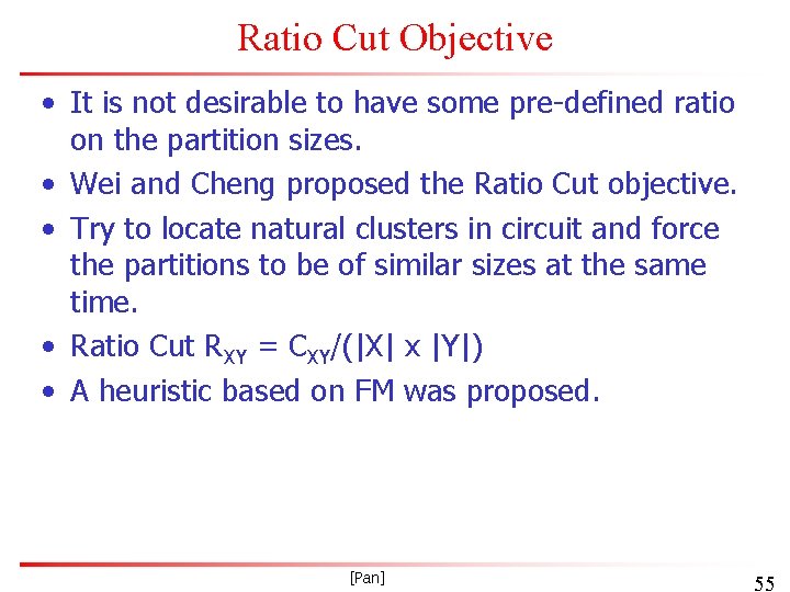
Ratio Cut Objective • It is not desirable to have some pre-defined ratio on the partition sizes. • Wei and Cheng proposed the Ratio Cut objective. • Try to locate natural clusters in circuit and force the partitions to be of similar sizes at the same time. • Ratio Cut RXY = CXY/(|X| x |Y|) • A heuristic based on FM was proposed. [Pan] 55

Sanchis Algorithm “Multiple-way Network Partitioning”, IEEE Trans. Computers, 38(1): 62 -81, 1989. [Pan] 56

Multi-Way Partitioning • Dividing into more than 2 partitions. • Algorithm by extending the idea of FM + Krishnamurthy. [Pan] 57

Simulated annealing • See text, section 2. 4. 4 58

Paper by Johnson, Aragon, Mc. Geoch and Schevon on Bisectioning using SA “Optimization by Simulated Annealing: An Experimental Evaluation Part I, Graph Partitioning”, Operations Research, 37: 865 -892, 1989. [Pan] 59

The Work of Johnson, et al. • An extensive empirical study of Simulated Annealing versus Iterative Improvement Approaches. • Conclusion: SA is a competitive approach, getting better solutions than KL for random graphs. Remarks: § Netlists are not random graphs, but sparse graphs with local structure. § SA is too slow. So KL/FM variants are still most popular. § Multiple runs of KL/FM variants with random initial solutions may be preferable to SA. [Pan] 60

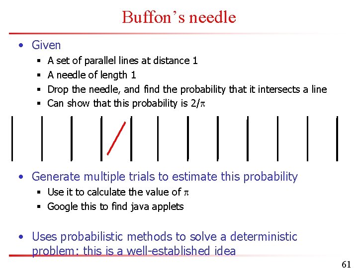
Buffon’s needle • Given § § A set of parallel lines at distance 1 A needle of length 1 Drop the needle, and find the probability that it intersects a line Can show that this probability is 2/ • Generate multiple trials to estimate this probability § Use it to calculate the value of § Google this to find java applets • Uses probabilistic methods to solve a deterministic problem: this is a well-established idea 61

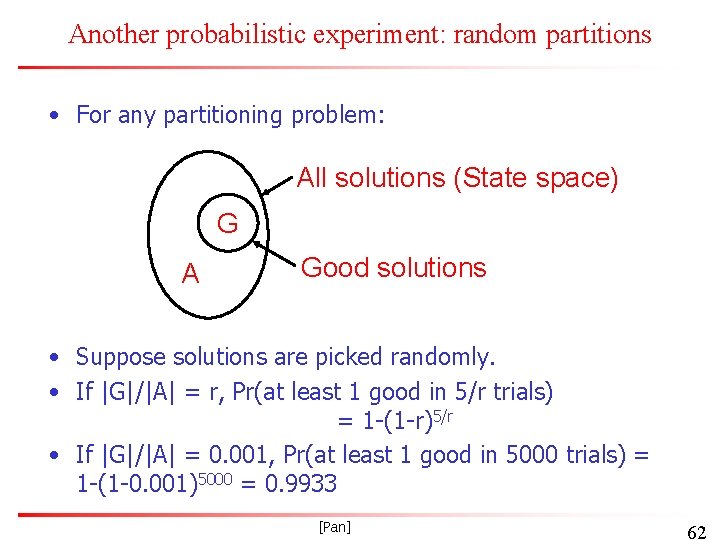
Another probabilistic experiment: random partitions • For any partitioning problem: All solutions (State space) G A Good solutions • Suppose solutions are picked randomly. • If |G|/|A| = r, Pr(at least 1 good in 5/r trials) = 1 -(1 -r)5/r • If |G|/|A| = 0. 001, Pr(at least 1 good in 5000 trials) = 1 -(1 -0. 001)5000 = 0. 9933 [Pan] 62

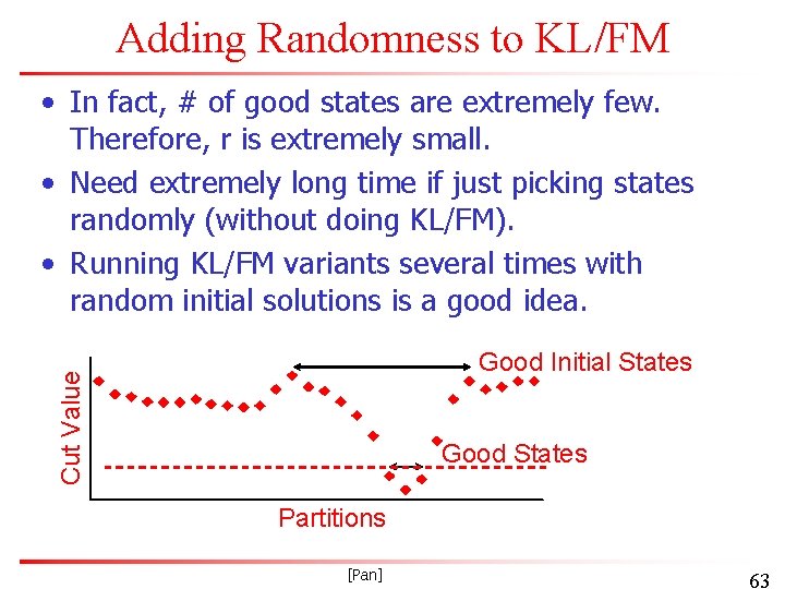
Adding Randomness to KL/FM • In fact, # of good states are extremely few. Therefore, r is extremely small. • Need extremely long time if just picking states randomly (without doing KL/FM). • Running KL/FM variants several times with random initial solutions is a good idea. Cut Value Good Initial States Good States Partitions [Pan] 63

Some Other Approaches • KL/FM-SA Hybrid: Use KL/FM variant to find a good initial solution for SA, then improve that solution by SA at low temperature. • Tabu Search • Genetic Algorithm • Spectral Methods (finding Eigenvectors) • Network Flows • Quadratic Programming • . . . [Pan] 64

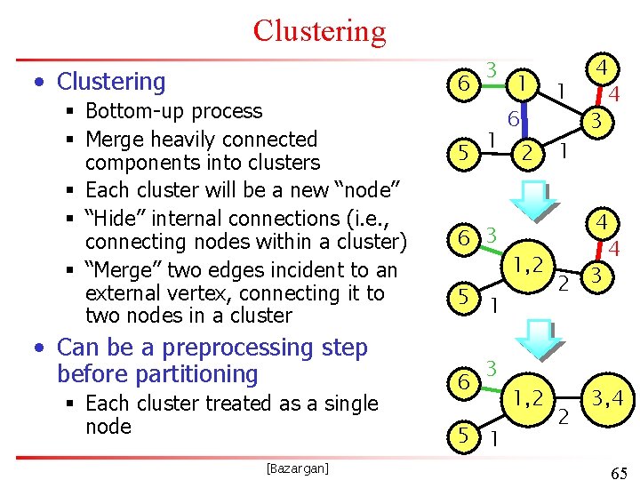
Clustering • Clustering § Bottom-up process § Merge heavily connected components into clusters § Each cluster will be a new “node” § “Hide” internal connections (i. e. , connecting nodes within a cluster) § “Merge” two edges incident to an external vertex, connecting it to two nodes in a cluster • Can be a preprocessing step before partitioning § Each cluster treated as a single node [Bazargan] 6 5 3 1 1 6 2 1 1 4 4 3 4 6 3 4 1, 2 2 3 5 1 6 3 5 1 1, 2 2 3, 4 65

Multilevel Hypergraph Partitioning: Applications in VLSI Domain G. Karypis, R. Aggarwal, V. Kumar and S. Shekhar, DAC 1997. [Pan] 66

Multi-Level Partitioning [Pan] 67

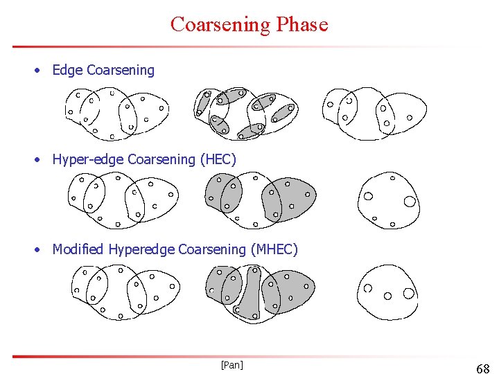
Coarsening Phase • Edge Coarsening • Hyper-edge Coarsening (HEC) • Modified Hyperedge Coarsening (MHEC) [Pan] 68

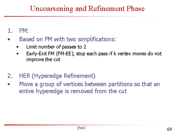
Uncoarsening and Refinement Phase 1. • FM: Based on FM with two simplifications: § § 2. • Limit number of passes to 2 Early-Exit FM (FM-EE), stop each pass if k vertex moves do not improve the cut HER (Hyperedge Refinement) Move a group of vertices between partitions so that an entire hyperedge is removed from the cut [Pan] 69

h. METIS Algorithm • Software implementation available for free download from Web • h. METIS-EE 20 § § 20 random initial partitons with 10 runs using HEC for coarsening with 10 runs using MHEC for coarsening FM-EE for refinement • h. METIS-FM 20 § § 20 random initial partitons with 10 runs using HEC for coarsening with 10 runs using MHEC for coarsening FM for refinement [Pan] 70

Experimental Results • Compared with five previous algorithms • h. METIS-EE 20 is: § 4. 1% to 21. 4% better § On average 0. 5% better than the best of the 5 algorithms § Roughly 1 to 15 times faster • h. METIS-FM 20 is: § On average 1. 1% better than h. METIS-EE 20 § Improves the best-known bisections for 9 out of 23 test circuits § Twice as slow as h. METIS-EE 20 [Pan] 71