Partitioned EliasFano Indexes Giuseppe Ottaviano Rossano Venturini ISTICNR

Partitioned Elias-Fano Indexes Giuseppe Ottaviano Rossano Venturini ISTI-CNR, Pisa Università di Pisa

Inverted indexes Docid Document 1: [it is what it is not] 2: [what is a] 3: [it is a banana] a banana is it not what 2, Posting 3 list 3 1, 2, 3 1 1, 2 • Core data structure of Information Retrieval • We seek fast and space-efficient encoding of posting lists (index compression)

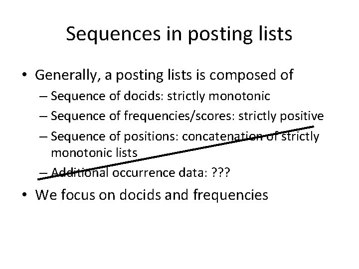
Sequences in posting lists • Generally, a posting lists is composed of – Sequence of docids: strictly monotonic – Sequence of frequencies/scores: strictly positive – Sequence of positions: concatenation of strictly monotonic lists – Additional occurrence data: ? ? ? • We focus on docids and frequencies

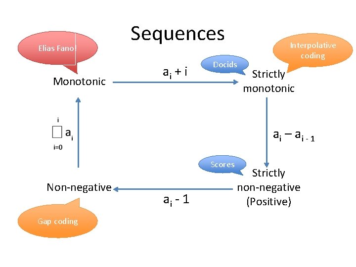
Elias Fano! Monotonic Sequences ai + i Docids Interpolative coding Strictly monotonic ai – a i - 1 Scores Non-negative Gap coding ai - 1 Strictly non-negative (Positive)

Elias-Fano encoding • Data structure from the ’ 70 s, mostly in the succinct data structures niche • Natural encoding of monotonically increasing sequences of integers • Recently successfully applied to inverted indexes [Vigna, WSDM 13] – Used by Facebook Graph Search!

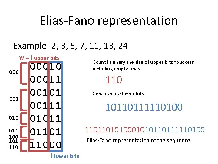
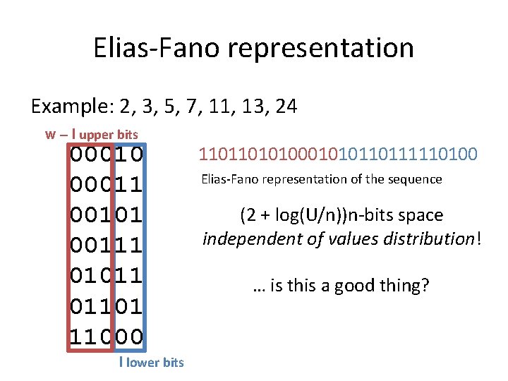
Elias-Fano representation Example: 2, 3, 5, 7, 11, 13, 24 w – l upper bits 000 001 010 011 100 101 110 00011 00101 00111 01011 01101 11000 l lower bits Count in unary the size of upper bits “buckets” including empty ones 11011010100010 Concatenate lower bits 10110111110100 1101101010001010110111110100 Elias-Fano representation of the sequence

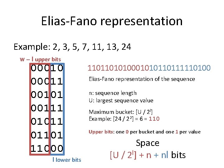
Elias-Fano representation Example: 2, 3, 5, 7, 11, 13, 24 w – l upper bits 00010 00011 00101 00111 01011 01101 11000 l lower bits 1101101010001010110111110100 Elias-Fano representation of the sequence n: sequence length U: largest sequence value Maximum bucket: [U / 2 l] Example: [24 / 22] = 6 = 110 Upper bits: one 0 per bucket and one 1 per value Space [U / 2 l] + nl bits

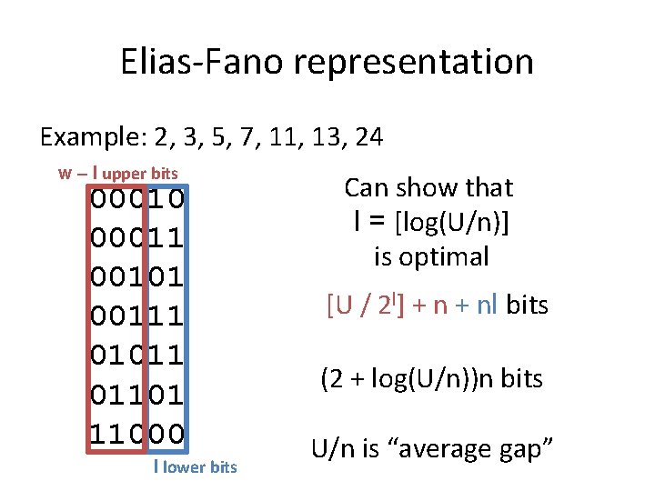
Elias-Fano representation Example: 2, 3, 5, 7, 11, 13, 24 w – l upper bits 00010 00011 00101 00111 01011 01101 11000 l lower bits Can show that l = [log(U/n)] is optimal [U / 2 l] + nl bits (2 + log(U/n))n bits U/n is “average gap”

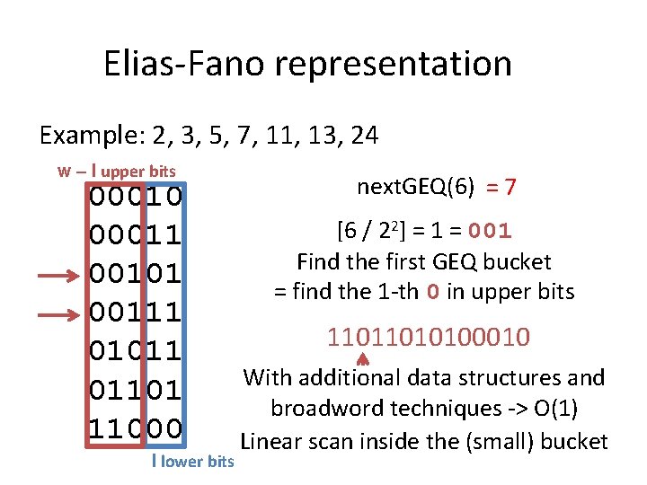
Elias-Fano representation Example: 2, 3, 5, 7, 11, 13, 24 w – l upper bits 00010 00011 00101 00111 01011 01101 11000 l lower bits next. GEQ(6) ? = 7 [6 / 22] = 1 = 001 Find the first GEQ bucket = find the 1 -th 0 in upper bits 11011010100010 With additional data structures and broadword techniques -> O(1) Linear scan inside the (small) bucket

Elias-Fano representation Example: 2, 3, 5, 7, 11, 13, 24 w – l upper bits 00010 00011 00101 00111 01011 01101 11000 l lower bits 1101101010001010110111110100 Elias-Fano representation of the sequence (2 + log(U/n))n-bits space independent of values distribution! … is this a good thing?

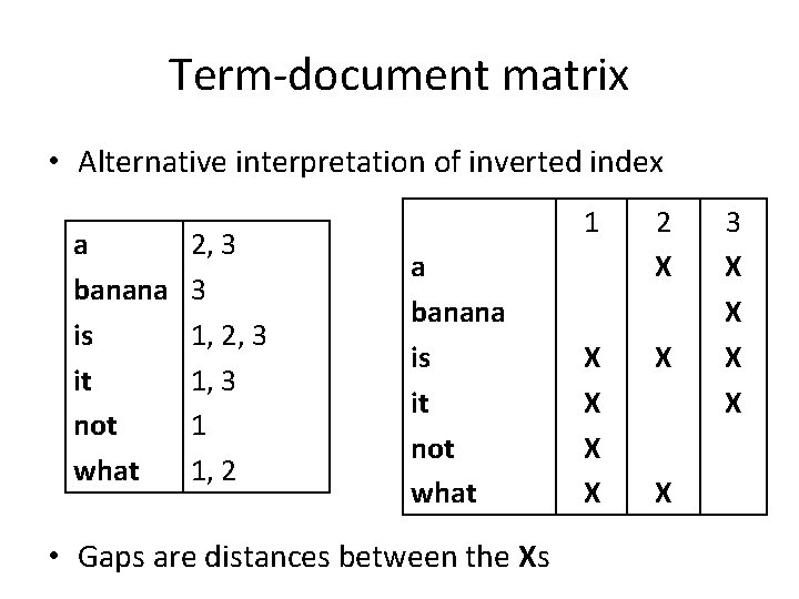
Term-document matrix • Alternative interpretation of inverted index a banana is it not what 2, 3 3 1, 2, 3 1 1, 2 a banana is it not what • Gaps are distances between the Xs 1 2 X X X X 3 X X

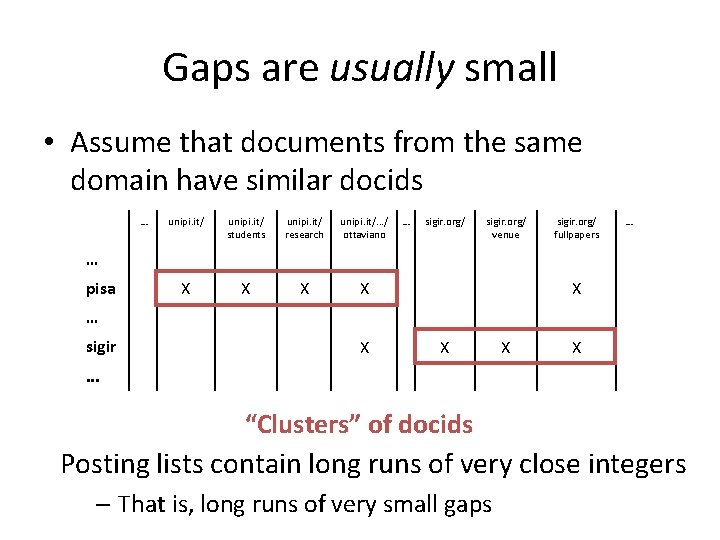
Gaps are usually small • Assume that documents from the same domain have similar docids … unipi. it/ students unipi. it/ research unipi. it/. . . / ottaviano X X … sigir. org/ venue sigir. org/ fullpapers … … pisa X … sigir X X . . . “Clusters” of docids Posting lists contain long runs of very close integers – That is, long runs of very small gaps

Elias-Fano and clustering • Consider the following two lists – 1, 2, 3, 4, …, n – 1, U – n random values between 1 and U • Both have n elements and largest value U – Elias-Fano compresses both to the exact same number of bits: (2 + log(U/n))n • But first list is far more compressible: it is “sufficient” to store n and U: O(log n + log U) • Elias-Fano doesn’t exploit clustering

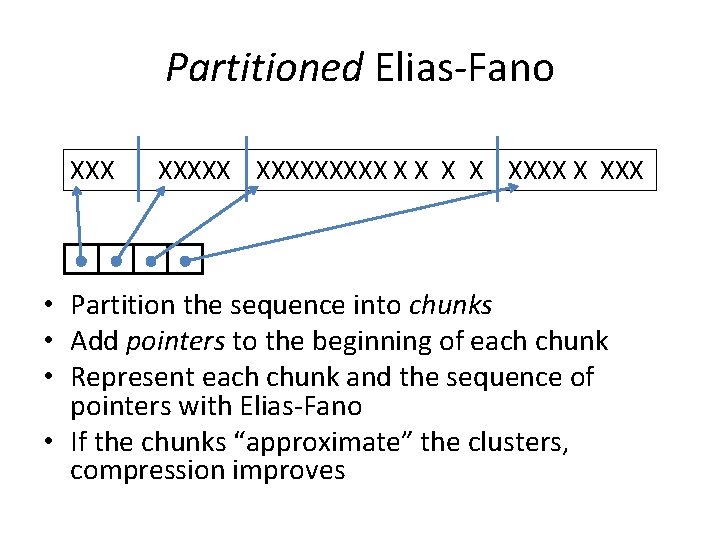
Partitioned Elias-Fano XXXXX X X XXXX X XXX • Partition the sequence into chunks • Add pointers to the beginning of each chunk • Represent each chunk and the sequence of pointers with Elias-Fano • If the chunks “approximate” the clusters, compression improves

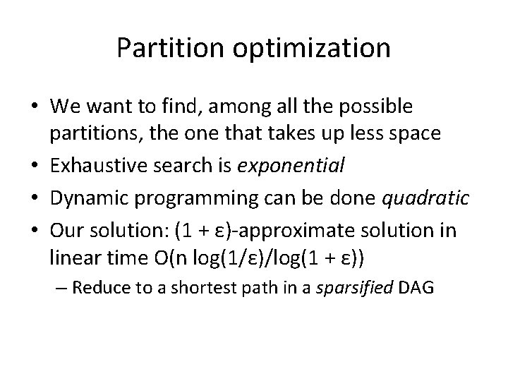
Partition optimization • We want to find, among all the possible partitions, the one that takes up less space • Exhaustive search is exponential • Dynamic programming can be done quadratic • Our solution: (1 + ε)-approximate solution in linear time O(n log(1/ε)/log(1 + ε)) – Reduce to a shortest path in a sparsified DAG

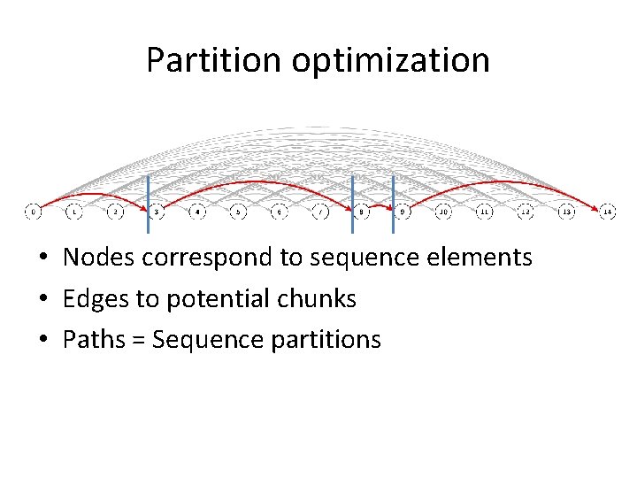
Partition optimization • Nodes correspond to sequence elements • Edges to potential chunks • Paths = Sequence partitions

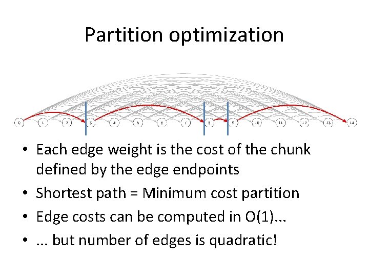
Partition optimization • Each edge weight is the cost of the chunk defined by the edge endpoints • Shortest path = Minimum cost partition • Edge costs can be computed in O(1). . . • . . . but number of edges is quadratic!

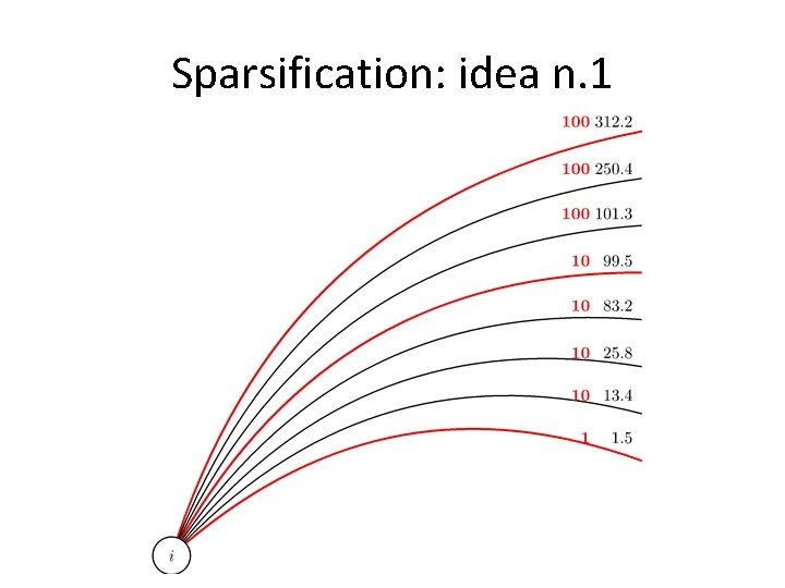
Sparsification: idea n. 1

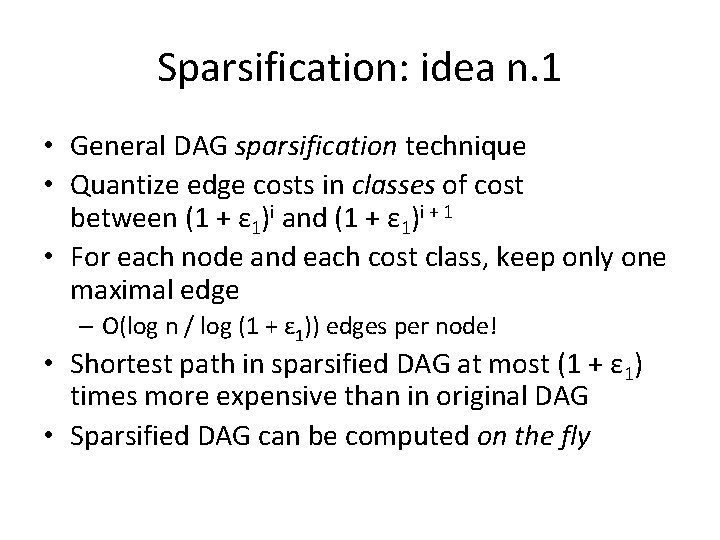
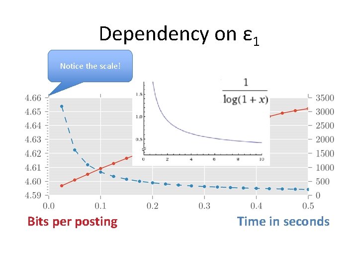
Sparsification: idea n. 1 • General DAG sparsification technique • Quantize edge costs in classes of cost between (1 + ε 1)i and (1 + ε 1)i + 1 • For each node and each cost class, keep only one maximal edge – O(log n / log (1 + ε 1)) edges per node! • Shortest path in sparsified DAG at most (1 + ε 1) times more expensive than in original DAG • Sparsified DAG can be computed on the fly

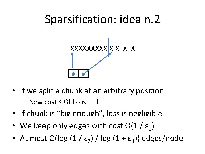
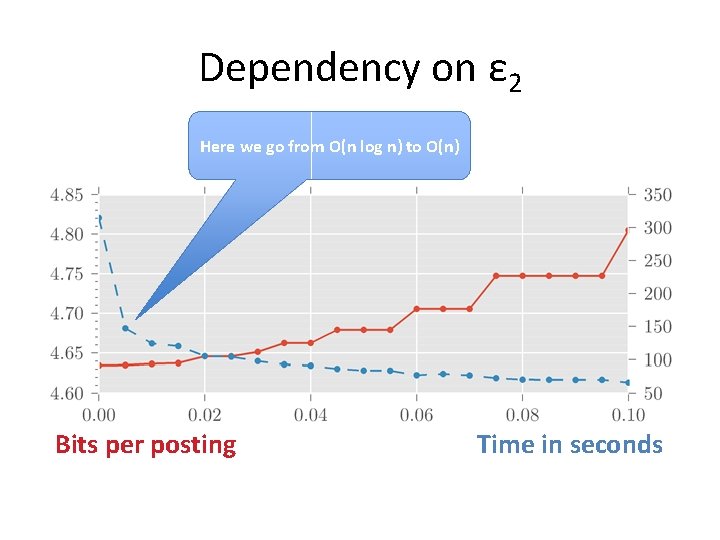
Sparsification: idea n. 2 XXXXX X X • If we split a chunk at an arbitrary position – New cost ≤ Old cost + 1 + cost of new pointer • If chunk is “big enough”, loss is negligible • We keep only edges with cost O(1 / ε 2) • At most O(log (1 / ε 2) / log (1 + ε 1)) edges/node

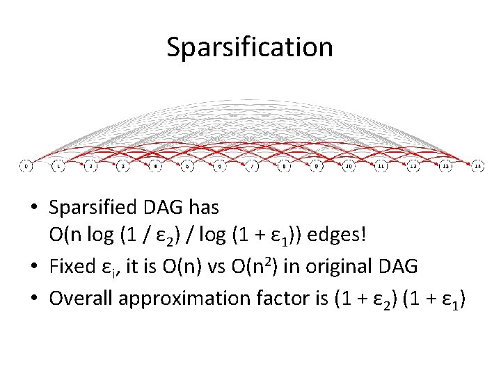
Sparsification • Sparsified DAG has O(n log (1 / ε 2) / log (1 + ε 1)) edges! • Fixed εi, it is O(n) vs O(n 2) in original DAG • Overall approximation factor is (1 + ε 2) (1 + ε 1)

Dependency on ε 1 Notice the scale! Bits per posting Time in seconds

Dependency on ε 2 Here we go from O(n log n) to O(n) Bits per posting Time in seconds

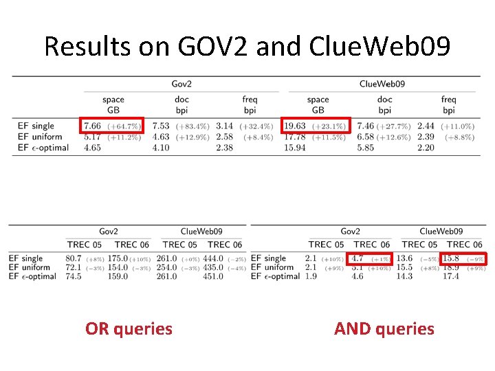
Results on GOV 2 and Clue. Web 09 OR queries AND queries

Thanks for your attention! Questions?